7. Compound Curves
a. Geometry
Sometimes a simple equal tangent vertical curve cannot be fit to a particular design condition. For example, the vertical curve in Figure B-24 must start at an existing intersection at sta 20+00 elev 845.25 ft and end at a second intersection at sta 28+00 elev 847.75 ft. To minimize earthwork an incoming grade of +2.50% is followed by an outgoing grade of -1.00%. This places the PVI at sta 23+00 elev 852.75 ft.
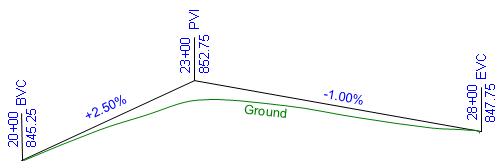 |
| Figure B-24 Fitting a Curve |
This combination results in a PVI that is not midway between the BVC and EVC. If a 600.00 ft equal tangent curve were used, it would begin at 20+00 and end at 26+00, 200.00 ft back along the -1.00% grade from the specified EVC.
This situation requires an unequal tangent vertical curve. While a mathematical curve other than a parabolic arc could be used, the traditional method is to use two back-to-back equal tangent curves. This is referred to as a compound curve, Figure B-25.
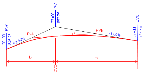 |
| Figure B-25 Compound Curve |
A compound curve isn't as complex as it looks: the key is to break it into two successive equal tangent veritical curves.
PVIs are created for each curve at midpoint on the grade lines. A new grade, g3, is created by connecting the new PVIs. This is the outgoing grade for the first curve and the incoming grade for the second.
The CVC is the Curve to Vertical Curve point which is the EVC of the first curve and the BVC of the second; its station is the same as the overall PVI station. Once we have sufficient information for each curve to set up its Curve Equation, we can compute each curve independently.
The closer the individual curve's k values, the smoother the transition between them, particularly when there is a large grade change over a short distance.
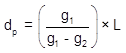
b. Curve Equation
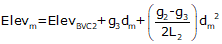
For an equal tangent vertical curve, we set up and solved Equations B-4 and B-5 through B-7. When setting these up for the curves in a compound curve, care must be taken to use the correct grades and lengths in each. Using subscripts i and m for the first and second curves respectively, their equations are:
| Curve 1 | Curve 2 | |
| Equation B-5 |  |
 |
| Equation B-7 | 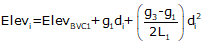 |
 |
| Equation B-8 |  |
 |
| Equation B-9 |  |
 |
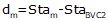
c. High/Low Point
A compound curve has the same high/low point condition as an equal tangent curve: it occurs where the curve grade passes through 0%.
For the compound curve shown in Figure B-24: the first curve has two positive grades so it never tops out, the second begins with a positive and ends with a negative grade. That places the highest point of this compound curve on the second curve.
When using the equation to compute distance to the low/high point, remember:
- use the grades for the curve on which the point occurs, and,
- the distance computed is from the BVC of the curve on which the point occurs.
For example, the distance equation Equation B-8 is:
 |
| Equation B-10 |
Setting up Equation B-10 and hi/low point station for each curve:
| Distance | Station | |
| Curve 1 | 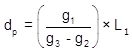 |
 |
| Curve 2 | 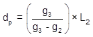 |
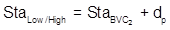 |
Remember: the high/low point occurs only on one curve or the other. Should g3 be 0%, then the low/high point would be at the CVC. If all three grades are positive or negative, then Equation B-10 does not apply as neither curve tops/bottoms out.
d. Example
Using the data given in Figure B-25:
(1) Complete the following table below
(2) Setup the Curve Equations for both curves
(3) Determine the station and elevation of the highest curve point.
Sketch
(1) Complete the table
|
Curve 1 |
Component |
Curve 2 |
|
incoming grade (%) |
||
|
outgoing grade (%) |
||
|
Length (ft) |
||
|
BVC Sta |
||
|
BVC Elev |
||
|
PVI Sta |
||
|
PVI Elev |
||
|
EVC Sta |
||
|
EVC Elev |
Entries that can be made from the given criteria:
|
Curve 1 |
Component |
Curve 2 |
| +2.50 |
incoming grade (%) |
|
|
outgoing grade (%) |
-1.00 | |
|
Length (ft) |
||
| 20+00 |
BVC Sta |
23+00 |
| 845.25 |
BVC Elev |
|
|
PVI Sta |
||
|
PVI Elev |
||
| 23+00 |
EVC Sta |
28+00 |
|
EVC Elev |
847.75 |
Compute:
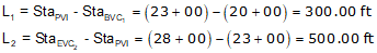
Since the PVIs are halfway along the grade lines, their positions are the averages of the grade line ends.
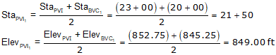
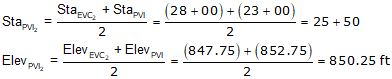
g3 is the grade of the line connecting the two curve PVIs. There can be different ways to compute it depending on the given data. In this example, we can use the position of the PVIs.
Compute the CVC elevation from PVI1.

The CVC elevation can also be computed from PVI2. We'll do it as a math check.

Complete the table.
|
Curve 1 |
Component |
Curve 2 |
| +2.50 |
incoming grade (%) |
+0.312 |
| +0.312 |
outgoing grade (%) |
-1.00 |
| 300.00 |
Length (ft) |
500.00 |
| 20+00 |
BVC Sta |
23+00 |
| 845.25 |
BVC Elev |
849.47 |
| 21+50 |
PVI Sta |
25+50 |
| 849.00 |
PVI Elev |
850.25 |
| 23+00 |
EVC Sta |
28+00 |
| 849.47 |
EVC Elev |
847.75 |
(2) Set up curve equations
Curve 1
Curve 2
Once these are set up, a Curve Table can be computed for each curve.
(3) Station and elevation of highest curve point.
The highest point will occur on Curve 2 since its grades go through 0%.
Use the equations for Curve 2.

e. Reverse Curve
A reverse curve is a compound curve except that the two curves have opposite curvature. It consists of either a sag-crest or crest-sag curves sequence, Figure B-26. The CRC (Curve to Reverse Curve) is the EVC of the first curve and BVC of the second.
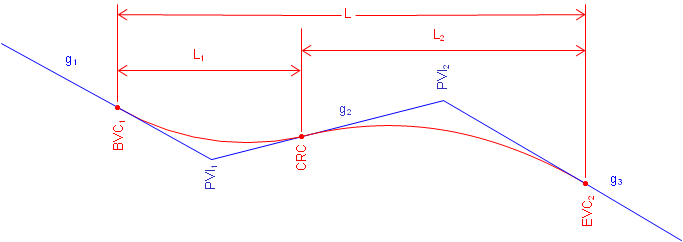 |
| Figure B-26 Reverse Curve |
Reverse vertical curves can be used to better approximate terrain to reduce earthwork. They also provide additional design flexibility if multiple design points are constrained. Their disadvantage is the vertical direction reversal which can be abrupt at higher speeds, particularly if the designer gets carried away and adds a third, fourth, etc, curve. Regardless, they are computed as equal tangent vertical curves once sufficient parameters for each is fixed or computed.
High/Low point determination can be interesting since both could exist on a reverse curve. For example, in Figure B-25, the first curve has a low point and the second has a high point. However, the lowest point on the entire curve is on the second curve at its EVC and the highest point on the entire curve is at the BVC of the first vertical curve.