a. Example 1
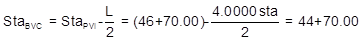
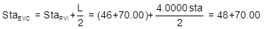
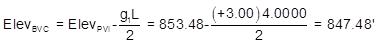
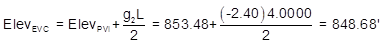
A +3.00% grade intersects a -2.40% at station 46+70.00 and elevation 853.48 ft. A 400.00 ft curve will be used to connect the two grades. Compute:
(1) Station and elevation for the curve's endpoints
(2) Elevations and grades at full stations
(3) Station and elevation of the curve's highest and lowest points
First, draw a sketch:
 |
| Figure B-15 Example 1 Sketch |
For our computations, we'll use grades in percent and distances in stations.
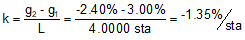
(1) Use Equations B-1 through B-4 to compute the BVC and EVC
 |
 |
 |
 |
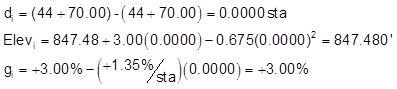
(2) Set up equations B-5, and B-7 to -9 to compute curve elevations.
|
Equation B-5 |
 |
| Equation B-7 | 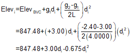 |
| Equation B-8 | 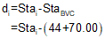 |
| Equation B-9 |  |
Set up the Curve Table:
| Equation B-8 |
Equation B-7 |
Equation B-9 |
|
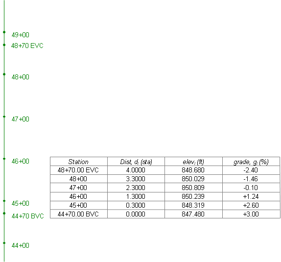
| Station, i | Dist, di (sta) | Elevi (ft) | Grade, gi (%) |
| 48+70.00 EVC | |||
| 48+00 | |||
| 47+00 | |||
| 46+00 | |||
| 45+00 | |||
| 44+70.00 BVC |
Why is the table upside down? We'll get to that in a second.
For each station, starting at the BVC, compute each column using the equation identified at the column top. Elevations will be computed to an additional decimal place to minimize rounding error.
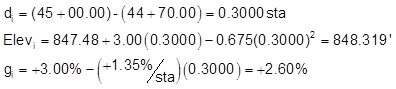
sta 44+70.00:
sta 45+00:
and so on to the EVC. At the EVC each computed value has a math check indicated in red.
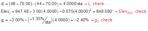
sta 48+70.00:
The completed Curve Table:
| Equation B-8 |
Equation B-7 |
Equation B-9 |
|
| Station, i | Dist, di (sta) | Elevi (ft) | Grade, gi (%) |
| 48+70.00 EVC | 4.0000 | 848.680 | -2.40 |
| 48+00 | 3.3000 | 850.029 | -1.46 |
| 47+00 | 2.3000 | 850.809 | -0.10 |
| 46+00 | 1.3000 | 850.239 | +1.24 |
| 45+00 | 0.3000 | 848.319 | +2.60 |
| 44+70.00 BVC | 0.0000 | 847.480 | +3.00 |
There are a few other math checks in addition to those at the EVC.
In the Dist column, the difference between successive d's at full stations should be 1.0000
In the Grade column, the difference between successive g's at full stations should be k=-1.35
Some texts make reference to Second Differences or Double Differences as another check. When computations were all done manually, as many checks as possible were used. We'll include it here just to show the reader how it worked.
A Second Difference is the difference between the elevation differences at full stations. Difference of a difference, got it? For this problem, we compute second differences this way:
|
Station |
Elevi (ft) |
First Difference |
Second Difference |
|
48+70.00 EVC |
848.680 |
|
|
|
48+00 |
850.029 |
850.029-850.809=-0.780 |
-0.780-0.570=-1.350 |
|
47+00 |
850.809 |
850.809-850.239=+0.570 |
+0.570-1.920=-1.350 |
|
46+00 |
850.239 |
850.239-848.319=+1.92 |
|
|
45+00 |
848.319 |
|
|
|
44+70.00 BVC |
847.480 |
|
|
Note that values in the Second Difference column are equal to k, that's the math check. For you calculus buffs, the second difference is the second derivative of the Curve Equation.
It looks like a lot of computing for only two checks against k (and it is). But for those two checks to be valid requires that 5 of the 7 elevations be correct. The remaining two are the BVC and EVC.
BTW, had we computed the curve elevations at half station intervals (every 50 ft), the double differences would be k/2.
(3) High and low point
Because this is a crest curve it will have a high point somewhere along it. The lowest point of the curve is at the BVC: 847.48 ft at 44+70.00.
Examining elevations in the completed Curve Table, it looks like the curve tops out between stations 46+00 and 48+00.
Use Equation B-10 to compute the distance from the BVC:
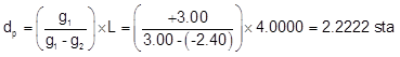
Substitute into the Curve Equation to determine its elevation:

Add the distance to the BVC station to get the point's station:
In summary
|
Point |
Station |
Elevation (ft) |
|
High |
46+92.22 |
850.81 |
|
Low |
44+70.00 BVC |
847.48 |
(4) Midpoint
Another math check is computing the curve midpoint elevation two ways
First using the curve equation

Then using offsets

(5) Misc
You're not restricted to computing elevations only at full stations along the curve. Using the equations in step (2) developed for this curve, you can compute the elevation and grade for any point between 0.00' and 400.00' feet from the BVC. If you exceed 400.00', the equations will give you values (after all, they're just equations), but for part of the curve beyond.
OK, so why the upside down table? It's traditional. When standing on the alignment and looking up station, the layout of the table visually matches the stations in front of the surveyor, Figure B-16.
 |
| Figure B-16 Upside Down Curve Table |