B. Vertical Curves

1. Nomenclature

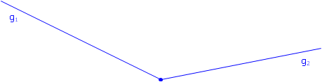
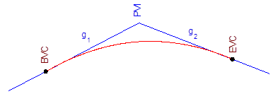
A vertical curve is used to provide a smooth transition between two different grade lines, Figure B-1.

Figure B-1 Adding a Vertical Curve

 

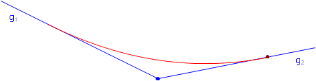
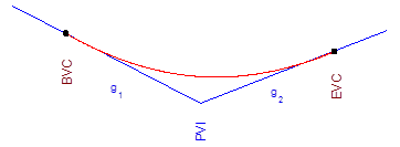
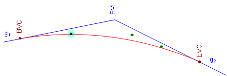
The parts of the curve, Figure B-2, are:

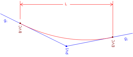Figure B-2 Curve Parts

 

PVI	Point of Vertical Intersection (aka PI)
BVC	Begin Vertical Curve (aka, BC, PVC, PC)
EVC	End Vertical Curve (aka EC, PVT, PT)
L	Curve Length

 

Distances, including the curve length, are horizontal, not along the grade lines or curve.

An equal tangent vertical curve is used. This places BVC and EVC equidistant from the PVI, Figure B-3.

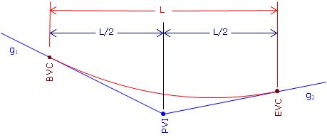Figure B-3 Equal Tangent Vertical Curve

 

The curve is tangent to the grade lines at both ends to provide a smooth transition between the grade lines and curve.

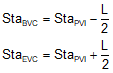
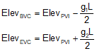
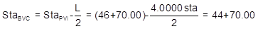
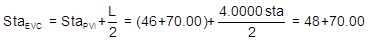
The stations and elevations of the BVC and EVC are determined from Equations B-1, -2, -3, and -4.

Equations B-1 and B-2		Equations B-3 and B-4

 

Because grade ratio and percent differ by a factor of 100 as do distances in feet or stations, care must be taken to use the correct form of each in Equations B-1 through  B-4. If g is in %, then L must be in stations, if g is a ratio, then L is in feet.

2. Grade Change Rate

A vehicle enters the curve at g₁ and after a distance of L it departs the curve at g₂. The total grade change is (g₂-g₁). The grade change rate, k, is the total grade change divided by the distance, Equation B-5.

Equation B-5

 

For example, a -2.00% grade into a +1.00% grade connected with a 400.00 ft curve has a k of:

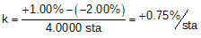
This tells us that the grade changes +0.75% per each 100 ft of curve. If we go 100 ft past the BVC, the curve grade is -1.00%+0.75% = +0.25%

Increasing the curve length to 900.00 ft changes k to +0.33%/sta.

The second smaller k means the longer curve is flatter since is spreads the total grade change over a longer distance, Figure B-4.

Figure B-4 Different Curve Lengths

 

Note that the example was a sag curve with a positive k: we went from a negative grade to a positive grade. A crest curve, on the other hand, would have a negative grade change rate, Figure B-5.

Figure B-5 Crest and Sag Curves

 

What about curves whose grades at both ends are different but have the same mathematical sign? Figure B-6 shows four different curve situations where the incoming and outgoing grades have the same mathematical sign.

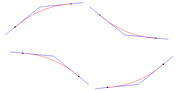Figure B-6 Grades with Same Mathematical Sign

 

The two curves on the left are both crest curves having a negative k since the outgoing grades are less than the incoming grades.

The two curves on the right are sag curves having a positive k since their outgoing grades are mathematically greater (less negative or more positive) than the incoming grades.

3. Curve Equation

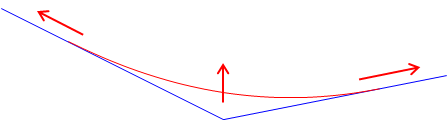
A constant grade change rate means the curve does not have a fixed radius - it's continually changing. This provides a smoother transition when vertical travel direction is changed. A circular arc isn't generally used as a vertical curve because it has constant curvature with a fixed radius. While acceptable at lower speeds, at higher speeds there is a tendency for a vehicle to "fly" at the highest point of a crest curve or "bottom out" at the lowest point of a sag curve. While desirable for roller coaster design, upsetting passenger stomachs is generally frowned upon in road design.

Instead, a parabolic arc is used. A parabola tends to flatten at the vertical direction change making for a more comfortable transition.

The general equation for a parabolic curve, Figure B-7, is Equation B-6.

	Equation B-6
Figure B-7 Parabola

 

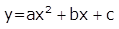
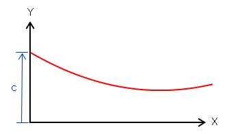
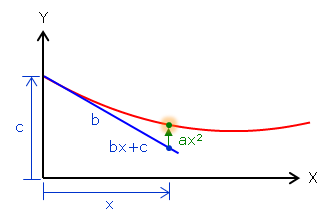
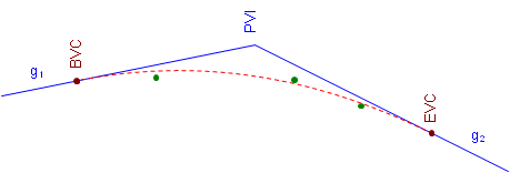
The equation consists of two parts, Figure B-8:

• a straight line, bx+c, which is tangent to the curve at its beginning (b is the slope, c is the y intercept), and,
• an offset, ax², which is the vertical distance from the tangent to the curve.

Figure B-8 Tangent and Offset

 

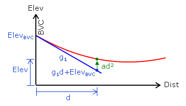
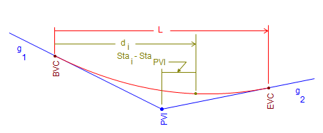
Figure B-9 shows the parabolic arc in terms of vertical curve nomenclature.

Figure B-9 Curve Terms

 

The curve begins at the BVC station and elevation.
The tangent line slope is g₁, the incoming grade.

At distance d:

• the tangent elevation is g₁d+Elev_BVC
• the tangent offset is ad², where a is a function of k

The parabolic equation written in curve terms is the Curve Equation, Equation B-7.

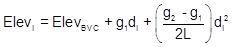Equation B-7

(For a complete graphic derivation of the Curve Equation see the Family of Curves section.)

d_i is the distance from the BVC to any point i on the curve. It is computed from Equation B-8 and ranges from 0 to L.

Equation B-8

Recall the previous warning on grade and distance units. In Equation B-5 the combination should be either grades in percent with distances in stations, or grades as a ratio with distances in feet. Remember that curve length, L, is a distance and must play by the same rules.

The grade at any point on the curve is a function of the beginning grade along with k and the distance from the BVC, Equation B-9.

Equation B-9

 

Using Equations B-7 through B-9 allows us to compute the elevation and grade at any point along the curve.  To compute the elevation of the curve's midpoint, L/2 would be used for d_i in Equation B-7.

A geometric characteristic of a parabolic vertical curve is at its midpoint the vertical offsets from the PVI to the curve and from the curve to the chord, o in Figure B-10, are the same.

Figure B-10 Midcurve Offsets

 

Besides using Equation B-7, another way to compute the midpoint elevation is from the following:

• The chord's midpoint elevation is the average elevation of the BVC and EVC.
• The curve's midpoint elevation is the average elevation of the chord midpoint and PVI.

The curve midpoint generally isn't any more or less important than other curve points. Being able to compute its elevation two ways, however, can be used as a partial math check

4. High or Low Point

When asked where a curve's highest, or lowest, point is, most people assume it is at the middle of the curve. This is true only under a specific condition. The high or low point occurs where the curve changes direction vertically. This happens where the curve tangent has a 0% grade, Figure B-11.

a. Crest Curve

b. Sag Curve

Figure B-11 High and Low Point Conditions

 

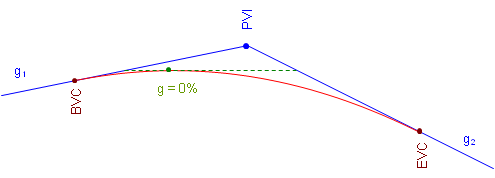
On a crest curve, the tangent grade begins at g₁ and deceases uniformly (by k). As long as the grade is positive, the curve elevation keeps increasing. At 0%, the curve reaches its maximum elevation and after that the grade decreases, causing curve elevations to drop.

The opposite is true for a sag curve. As the grade decreases, while it is still negative curve elevations decrease. When the grade is 0%, the elevation decrease stops and as the tangent slope increases so do curve elevations.

The only condition under which the high or low point occurs at the center of the curve is when incoming and outgoing grades are numerically equal but have opposite mathematical signs (eg, +2% into -2%, -3% into +3%).

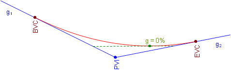
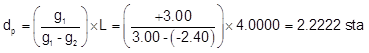
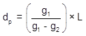
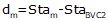
The distance from the BVC to the high/low point, d_p in Figure B-12, is determined from Equation B-10:

		Equation B-10
Figure B-12 Distance to High/Low Point

The high/low point elevation can be computed by substituting d_p in Equation B-7.

In order for Equation B-8 to return a value that makes sense, the grades must have opposite mathematical signs. Consider a +3.00% grade connected to a +1.00% grade with a 500.00 ft long curve. Using Equation B-10 the distance from the BVC to the high/low point is:

The distance exceeds the curve length. What's up with that? Let's sketch it, Figure B-13.

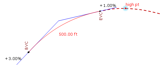Figure B-13 High Point After the EVC

Remember, we are using only part of the parabolic curve. 7.5000 stations is the distance to the curve's highest point, it's just on that part of the curve we're not using. Our curve's actual highest point is at the EVC.

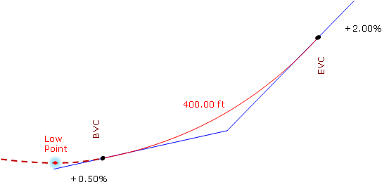
Similarly for a +0.50% grade connected to a +2.00% with a 400.00 ft curve:

This means the high/low point occurs before the BVC, Figure B-14.

Figure B-14 Low Point Before the BVC

The lowest point for this curve is at the BVC.

 

5. Example Problems

Vertical curve computations aren't as complicated as they may seem. The keys are to determine endpoints and set up the curve equation. From there it's just repetitious solution of the curve equation. 

a. Example 1

A +3.00% grade intersects a -2.40% at station 46+70.00 and elevation 853.48 ft. A 400.00 ft curve will be used to connect the two grades. Compute:

(1) Station and elevation for the curve's endpoints
(2) Elevations and grades at full stations
(3) Station and elevation of the curve's highest and lowest points

First, draw a sketch:

Figure B-15 Example 1 Sketch

 

For our computations, we'll use grades in percent and distances in stations.

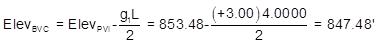
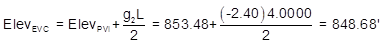
(1) Use Equations B-1 through B-4 to compute the BVC and EVC

 

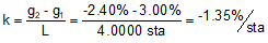
(2) Set up equations B-5, and B-7 to -9 to compute curve elevations.

Equation B-5
Equation B-7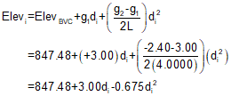
Equation B-8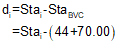
Equation B-9

 

 Set up the Curve Table:

Curve Table

	Equation B-8	Equation B-7	Equation B-9
Station, i	Dist, di (sta)	Elevi (ft)	Grade, gi (%)
48+70.00 EVC
48+00
47+00
46+00
45+00
44+70.00 BVC

 

Why is the table upside down? We'll get to that in a second.

For each station, starting at the BVC, compute each column using the equation identified at the column top. Elevations will be computed to an additional decimal place to minimize rounding error.

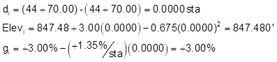
sta 44+70.00:

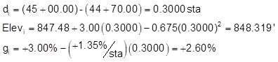
sta 45+00:

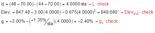
and so on to the EVC. At the EVC each computed value has a math check indicated in red.

sta 48+70.00:

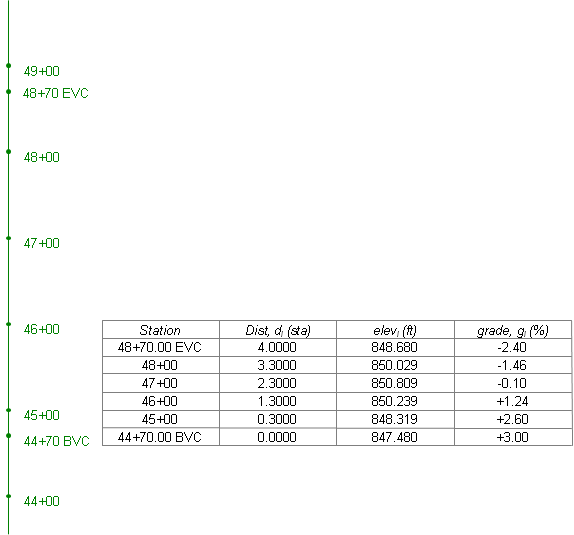
The completed Curve Table:

Curve Table

	Equation B-8	Equation B-7	Equation B-9
Station, i	Dist, di (sta)	Elevi (ft)	Grade, gi (%)
48+70.00 EVC	4.0000	848.680	-2.40
48+00	3.3000	850.029	-1.46
47+00	2.3000	850.809	-0.10
46+00	1.3000	850.239	+1.24
45+00	0.3000	848.319	+2.60
44+70.00 BVC	0.0000	847.480	+3.00

 

There are a few other math checks in addition to those at the EVC.

In the Dist column, the difference between successive d's at full stations should be 1.0000

In the Grade column, the difference between successive g's at full stations should be k=-1.35

Some texts make reference to Second Differences or Double Differences as another check. When computations were all done manually, as many checks as possible were used. We'll include it here just to show the reader how it worked.

A Second Difference is the difference between the elevation differences at full stations. Difference of a difference, got it? For this problem, we compute second differences this way:

Station	Elevi (ft)	First Difference	Second Difference
48+70.00 EVC	848.680
48+00	850.029	850.029-850.809=-0.780	-0.780-0.570=-1.350
47+00	850.809	850.809-850.239=+0.570	+0.570-1.920=-1.350
46+00	850.239	850.239-848.319=+1.92
45+00	848.319
44+70.00 BVC	847.480

 

Note that values in the Second Difference column are equal to k, that's the math check. For you calculus buffs, the second difference is the second derivative of the Curve Equation.

It looks like a lot of computing for only two checks against k (and it is). But for those two checks to be valid requires that 5 of the 7 elevations be correct. The remaining two are the BVC and EVC.

BTW, had we computed the curve elevations at half station intervals (every 50 ft), the double differences would be k/2.

(3) High and low point

Because this is a crest curve it will have a high point somewhere along it. The lowest point of the curve is at the BVC: 847.48 ft at 44+70.00.

Examining elevations in the completed Curve Table, it looks like the curve tops out between stations 46+00 and 48+00.

Use Equation B-10 to compute the distance from the BVC:

Substitute into the Curve Equation to determine its elevation:

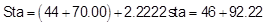
Add the distance to the BVC station to get the point's station:

In summary

Point	Station	Elevation (ft)
High	46+92.22	850.81
Low	44+70.00 BVC	847.48

 

(4) Midpoint

Another math check is computing the curve midpoint elevation two ways

First using the curve equation

Then using offsets

(5) Misc

You're not restricted to computing elevations only at full stations along the curve. Using the equations in step (2) developed for this curve, you can compute the elevation and grade for any point between 0.00' and 400.00' feet from the BVC. If you exceed 400.00', the equations will give you values (after all, they're just equations), but for part of the curve beyond.

OK, so why the upside down table? It's traditional. When standing on the alignment and looking up station, the layout of the table visually matches the stations in front of the surveyor, Figure B-16.

Figure B-16 Upside Down Curve Table

 

b. Example 2

A -3.50% grade intersects a +2.00% at station 12+17.53 and elevation 634.25 ft. A 400.00 ft curve will be used to connect the two grades. Compute:

(1) Station and elevation for the curve's endpoints
(2) Elevations and grades at half stations
(3) Station and elevation of the curves highest and lowest points

The computations are left to the reader. The answers are shown for checking your work.

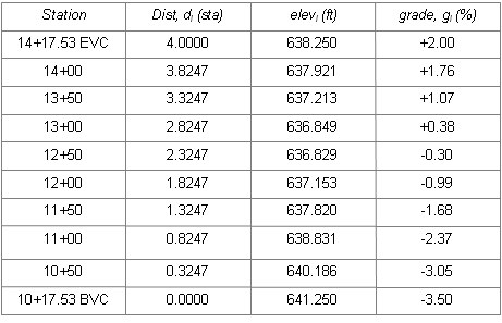
Low point at sta 12+72.07 and elev 636.80 ft.

6. Fitting Vertical Curves

a. Introduction

There are many different combinations of fitting a vertical curve to meet design conditions. In this section we will concentrate on two examples of fitting an equal tangent curve between fixed grade lines. Holding grade lines fixed isolates curve selection effects. When a grade is changed, whole sections of the alignment are affected and must be recomputed, Figure B-17. Although software can easily handle this, it's the designer's responsibility to ensure solving a problem in one area doesn't adversely affect another.

(a) Preliminary Vertical Alignment

(b) Holding Grades Fixed

(c) Changing a Grade

Figure B-17 Fitting Vertical Curves

 

In these examples we will compute simple equal tangent curves to meet some elevation condition between fixed grade lines. The next section deals with unequal tangent vertical curves which give additional design flexibility but at the cost of more complex computations.

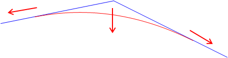
When computing a curve passing through an elevation, the computed length may be a maximum or minimum. It depends if the specified elevation is a maximum or minimum and whether a sag or crest curve is involved. Increasing the length of a sag curve raises the entire curve; increasing a crest curve's length lowers it, Figure B-18.

(a) Increasing Sag Curve Length

(b) Increasing Crest Curve Length

Figure B-18 Curve Length and Elevations

 

To solve lengths requires rearranging and solving the Curve Equation, Equation B-7, for the unknown L.

Equation B-7

It looks simple until you realize that d_i is dependent on the location of the BVC which is in turn based on the curve length we're tying to compute. Hmmm....

b. No part of a curve may go below {above} a specific elevation

This criteria could come from the elevation of area groundwater, bedrock, or an existing overhead pass. The critical curve part of for this situation is the curve's highest or lowest point, Figure B-19.

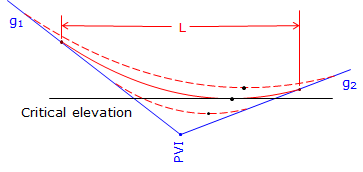Figure B-19 Low Point Condition

 

The distance to the high/low point was given in Equation B10:

Equation B-10

 

Substituting Equation B-10 into Equation B-7 and solving for L, we arrive at Equation B-9:

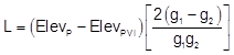Equation B-11

 Remember: grades in % and L in stations.

Example

g₁ & g₂ are -5.00% and +2.00% respectively; the PVI is at 10+00.00 with an elev of 800.00 ft.

What is the length of curve which does not go below 805.00 ft elev? Is this a maximum or minimum curve length?

Draw a sketch:

Substitute known data into Equation B-11 and solve:

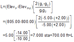
The curve should be at least 700.00 ft long. Using a longer length is fine since it raises the curve up from 805.00 ft.

Are there any math checks?

Using L=700.00 ft, set up the Curve Equation and compute the low point's elevation.

 

c. Curve must pass thru a specific elevation at a specific station

In this case the curve has to pass through a particular elevation at a particular station. For example, an existing road crossing may dictate the station and elevation for an at-grade intersection.

This situation appears to be easier since, unlike the previous example, we know the station at which the elevation must be met, Figure B-20.

Figure B-20 Elevation at a Station

 

Since we know the station of the fixed elevation, we can determine its distance from the PVI. We can also relate the BVC location to the PVI.
If we substitute known and related quantities into Equation B-5, we get:

Equation B-12

 

OK, maybe it's not as simple as it seemed. But the only unknown in the equation is L; unfortunately, it appears as numerator and denominator in the various terms. If we combine and sort terms we see that the equation takes on the form of a (surprise!) parabolic equation, a second degree polynomial. A second degree polynomial has two solutions and can be solved using the quadratic solution.

Second Degree Polynomial Equation B-13(a)	Quadratic Solution Equation B-13(b)

 

 To simplify Equation B-10 and solve it using the quadratic solution we can create the following two sets of equations:

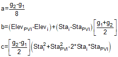Quadratic Coefficients Equations B-14, B-15, and B-16	Curve Length Solutions      Equation B-17

 

Equation B-17 will return two values for the curve length, one which makes sense in the context of the problem, the other which doesn't.

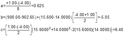
Example

g₁ & g₂ are -4.00% and +1.00% respectively, the PVI is at 14+00.00 with an elev of 900.00 ft.
The curve must go through an elevation of 902.65 at station 15+60.00.
What curve length meets this condition?

Draw a sketch

Compute the quadratic coefficients using Equation B-14, -15, -16:

Compute the curve lengths using Equation B-17:

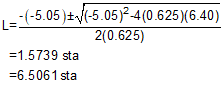
Which curve length is correct?

Compute the BVC and EVC stations for each curve length and see if station 15+60.00 falls between them.

Length (sta)	BVC Sta	EVC Sta	15+60 bewteen?
1.5739	13+21.30	14+78.70	No
6.5061	10+74.70	17+25.30	Yes

 The correct curve length is 650.61 ft.

Math check?

Set up the Curve Equation, Equation B-7, and solve for the elevation at station 15+60.00. It should be the same as the specified elevation of 902.65 ft.

Why are there two possible curve lengths and why does only one fit our design situation?

Remember that these are mathematical formulae independent of physical constraint. We are using only part of a complex curve for our alignment design which does have physical constraints.

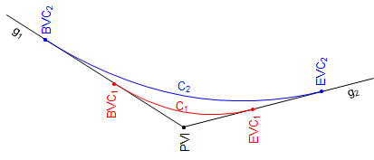
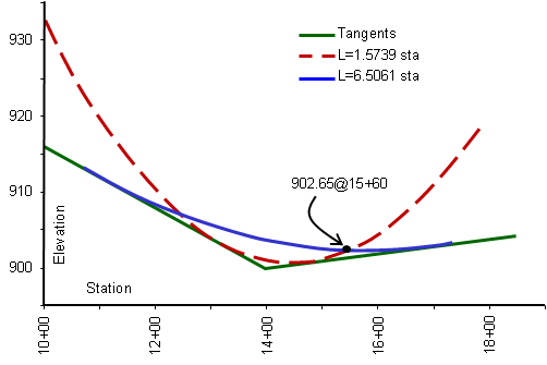
There are two parabolic curves which are tangent to the grade lines and pass through the design point. These are shown plotted in Figure B-21.

Figure B-21 Two Curve Solutions

 

Both curves are tangent to the two grade lines and pass through sta 15+60 and elev 902.65. Only one of the curves has the design point between the tangent (BVC and EVC) points on the grade lines. Mathematically both curves are correct, but only one meets our design criteria.

d. Multiple design points

It may not be possible to design an equal tangent curve to pass through multiple design points, Figure B-22. A single curve can be fit if each of the points can be missed by a specified amount. Least squares could be applied in this case to create a best-fit curve.

Figure B-22 Multiple Design Points

 

Or one of the points could be treated as the most critical and used to design a curve, Figure B-23.

Figure B-23 Critical Point Fit

 

Another possible approach is to use a compound vertical curve which will be covered next.

e. Spreadsheet

An Excel spreadsheet to fit a vertical curve based on high/low point or station and elevation can be downloaded here. It uses Visual Basic for Applications script so Excel must have macros enabled when loading the sheet.

7. Compound Curves

a. Geometry

Sometimes a simple equal tangent vertical curve cannot be fit to a particular design condition. For example, the vertical curve in Figure B-24 must start at an existing intersection at sta 20+00 elev 845.25 ft and end at a second intersection at sta 28+00 elev 847.75 ft. To minimize earthwork an incoming grade of +2.50% is followed by an outgoing grade of -1.00%. This places the PVI at sta 23+00 elev 852.75 ft.

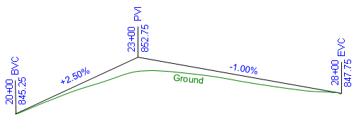Figure B-24 Fitting a Curve

 

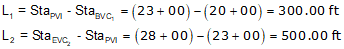
This combination results in a PVI that is not midway between the BVC and EVC. If a 600.00 ft equal tangent curve were used, it would begin at 20+00 and end at 26+00, 200.00 ft back along the -1.00% grade from the specified EVC.

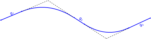
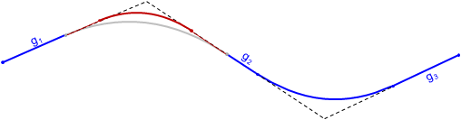
This situation requires an unequal tangent vertical curve. While a mathematical curve other than a parabolic arc could be used, the traditional method is to use two back-to-back equal tangent curves. This is referred to as a compound curve, Figure B-25.

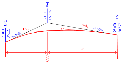Figure B-25 Compound Curve

 

A compound curve isn't as complex as it looks: the key is to break it into two successive equal tangent veritical curves.

PVIs are created for each curve at midpoint on the grade lines. A new grade, g₃, is created by connecting the new PVIs. This is the outgoing grade for the first curve and the incoming grade for the second.

The CVC is the Curve to Vertical Curve point which is the EVC of the first curve and the BVC of the second; its station is the same as the overall PVI station. Once we have sufficient information for each curve to set up its Curve Equation, we can compute each curve independently.

The closer the individual curve's k values, the smoother the transition between them, particularly when there is a large grade change over a short distance.

b. Curve Equation

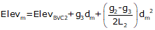
For an equal tangent vertical curve, we set up and solved Equations B-4 and B-5 through B-7. When setting these up for the curves in a compound curve, care must be taken to use the correct grades and lengths in each. Using subscripts i and m for the first and second curves respectively, their equations are:

	Curve 1	Curve 2
Equation B-5
Equation B-7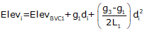
Equation B-8
Equation B-9

 

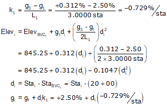
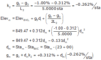
c. High/Low Point

A compound curve has the same high/low point condition as an equal tangent curve: it occurs where the curve grade passes through 0%.

For the compound curve shown in Figure B-24: the first curve has two positive grades so it never tops out, the second begins with a positive and ends with a negative grade. That places the highest point of this compound curve on the second curve.

When using the equation to compute distance to the low/high point, remember:

• use the grades for the curve on which the point occurs, and,
• the distance computed is from the BVC of the curve on which the point occurs.

For example, the distance equation Equation B-8 is:

Equation B-10

 

Setting up Equation B-10 and hi/low point station for each curve:

	Distance	Station
Curve 1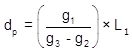
Curve 2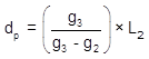

 

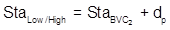Remember: the high/low point occurs only on one curve or the other. Should g₃ be 0%, then the low/high point would be at the CVC. If all three grades are positive or negative, then Equation B-10 does not apply as neither curve tops/bottoms out.

d. Example

Using the data given in Figure B-25:

(1) Complete the following table below
(2) Setup the Curve Equations for both curves
(3) Determine the station and elevation of the highest curve point.

Sketch

(1) Complete the table

Curve 1	Component	Curve 2
	incoming grade (%)
	outgoing grade (%)
	Length (ft)
	BVC Sta
	BVC Elev
	PVI Sta
	PVI Elev
	EVC Sta
	EVC Elev

 

Entries that can be made from the given criteria:

Curve 1	Component	Curve 2
+2.50	incoming grade (%)
	outgoing grade (%)	-1.00
	Length (ft)
20+00	BVC Sta	23+00
845.25	BVC Elev
	PVI Sta
	PVI Elev
23+00	EVC Sta	28+00
	EVC Elev	847.75

 

Compute:

 

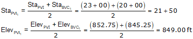
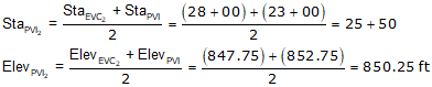
Since the PVIs are halfway along the grade lines, their positions are the averages of the grade line ends.

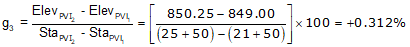
g₃ is the grade of the line connecting the two curve PVIs. There can be different ways to compute it depending on the given data. In this example, we can use the position of the PVIs.

Compute the CVC elevation from PVI₁.

The CVC elevation can also be computed from PVI₂. We'll do it as a math check.

Complete the table.

Curve 1	Component	Curve 2
+2.50	incoming grade (%)	+0.312
+0.312	outgoing grade (%)	-1.00
300.00	Length (ft)	500.00
20+00	BVC Sta	23+00
845.25	BVC Elev	849.47
21+50	PVI Sta	25+50
849.00	PVI Elev	850.25
23+00	EVC Sta	28+00
849.47	EVC Elev	847.75

 

(2) Set up curve equations

Curve 1

Curve 2

Once these are set up, a Curve Table can be computed for each curve.

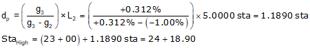
(3) Station and elevation of highest curve point.

The highest point will occur on Curve 2 since its grades go through 0%.

Use the equations for Curve 2.

 

e. Reverse Curve

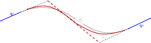
A reverse curve is a compound curve except that the two curves have opposite curvature. It consists of either a sag-crest or crest-sag curves sequence, Figure B-26. The CRC (Curve to Reverse Curve) is the EVC of the first curve and BVC of the second.

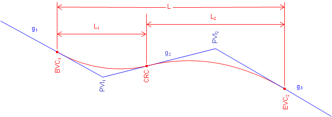Figure B-26 Reverse Curve

 

Reverse vertical curves can be used to better approximate terrain to reduce earthwork. They also provide additional design flexibility if multiple design points are constrained. Their disadvantage is the vertical direction reversal which can be abrupt at higher speeds, particularly if the designer gets carried away and adds a third, fourth, etc, curve. Regardless, they are computed as equal tangent vertical curves once sufficient parameters for each is fixed or computed.

High/Low point determination can be interesting since both could exist on a reverse curve. For example, in Figure B-25, the first curve has a low point and the second has a high point. However, the lowest point on the entire curve is on the second curve at its EVC and the highest point on the entire curve is at the BVC of the first vertical curve.