6. Fitting Vertical Curves
a. Introduction
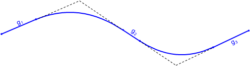
There are many different combinations of fitting a vertical curve to meet design conditions. In this section we will concentrate on two examples of fitting an equal tangent curve between fixed grade lines. Holding grade lines fixed isolates curve selection effects. When a grade is changed, whole sections of the alignment are affected and must be recomputed, Figure B-17. Although software can easily handle this, it's the designer's responsibility to ensure solving a problem in one area doesn't adversely affect another.
|
(a) Preliminary Vertical Alignment |
|
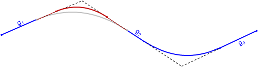
(b) Holding Grades Fixed |
|
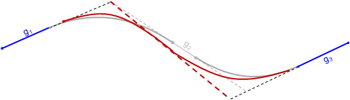
(c) Changing a Grade |
| Figure B-17 Fitting Vertical Curves |
In these examples we will compute simple equal tangent curves to meet some elevation condition between fixed grade lines. The next section deals with unequal tangent vertical curves which give additional design flexibility but at the cost of more complex computations.
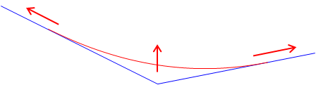
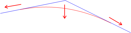
When computing a curve passing through an elevation, the computed length may be a maximum or minimum. It depends if the specified elevation is a maximum or minimum and whether a sag or crest curve is involved. Increasing the length of a sag curve raises the entire curve; increasing a crest curve's length lowers it, Figure B-18.
|
(a) Increasing Sag Curve Length |
|
(b) Increasing Crest Curve Length |
| Figure B-18 Curve Length and Elevations |
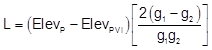
To solve lengths requires rearranging and solving the Curve Equation, Equation B-7, for the unknown L.
 |
| Equation B-7 |
It looks simple until you realize that di is dependent on the location of the BVC which is in turn based on the curve length we're tying to compute. Hmmm....
b. No part of a curve may go below {above} a specific elevation
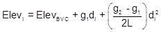
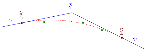
This criteria could come from the elevation of area groundwater, bedrock, or an existing overhead pass. The critical curve part of for this situation is the curve's highest or lowest point, Figure B-19.
 |
| Figure B-19 Low Point Condition |
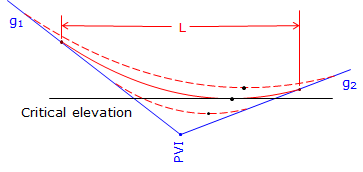
The distance to the high/low point was given in Equation B10:
 |
| Equation B-10 |
Substituting Equation B-10 into Equation B-7 and solving for L, we arrive at Equation B-9:
 |
| Equation B-11 |
Remember: grades in % and L in stations.
Example
g1 & g2 are -5.00% and +2.00% respectively; the PVI is at 10+00.00 with an elev of 800.00 ft.
What is the length of curve which does not go below 805.00 ft elev? Is this a maximum or minimum curve length?
Draw a sketch:

Substitute known data into Equation B-11 and solve:
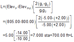
The curve should be at least 700.00 ft long. Using a longer length is fine since it raises the curve up from 805.00 ft.
Are there any math checks?
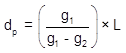
Using L=700.00 ft, set up the Curve Equation and compute the low point's elevation.
c. Curve must pass thru a specific elevation at a specific station
In this case the curve has to pass through a particular elevation at a particular station. For example, an existing road crossing may dictate the station and elevation for an at-grade intersection.
This situation appears to be easier since, unlike the previous example, we know the station at which the elevation must be met, Figure B-20.
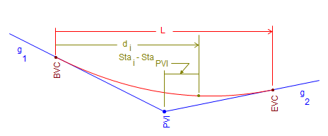 |
| Figure B-20 Elevation at a Station |
Since we know the station of the fixed elevation, we can determine its distance from the PVI. We can also relate the BVC location to the PVI.
If we substitute known and related quantities into Equation B-5, we get:
 |
| Equation B-12 |
OK, maybe it's not as simple as it seemed. But the only unknown in the equation is L; unfortunately, it appears as numerator and denominator in the various terms. If we combine and sort terms we see that the equation takes on the form of a (surprise!) parabolic equation, a second degree polynomial. A second degree polynomial has two solutions and can be solved using the quadratic solution.
|
|
|
| Second Degree Polynomial Equation B-13(a) |
Quadratic Solution |


To simplify Equation B-10 and solve it using the quadratic solution we can create the following two sets of equations:
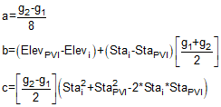 |
 |
| Quadratic Coefficients Equations B-14, B-15, and B-16 |
Curve Length Solutions Equation B-17 |
Equation B-17 will return two values for the curve length, one which makes sense in the context of the problem, the other which doesn't.
Example
g1 & g2 are -4.00% and +1.00% respectively, the PVI is at 14+00.00 with an elev of 900.00 ft.
The curve must go through an elevation of 902.65 at station 15+60.00.
What curve length meets this condition?
Draw a sketch

Compute the quadratic coefficients using Equation B-14, -15, -16:
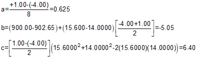
Compute the curve lengths using Equation B-17:
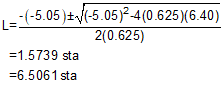
Which curve length is correct?
Compute the BVC and EVC stations for each curve length and see if station 15+60.00 falls between them.
| Length (sta) | BVC Sta | EVC Sta | 15+60 bewteen? |
| 1.5739 | 13+21.30 | 14+78.70 | No |
| 6.5061 | 10+74.70 | 17+25.30 | Yes |
The correct curve length is 650.61 ft.
Math check?
Set up the Curve Equation, Equation B-7, and solve for the elevation at station 15+60.00. It should be the same as the specified elevation of 902.65 ft.
Why are there two possible curve lengths and why does only one fit our design situation?
Remember that these are mathematical formulae independent of physical constraint. We are using only part of a complex curve for our alignment design which does have physical constraints.
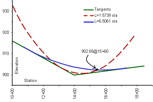
There are two parabolic curves which are tangent to the grade lines and pass through the design point. These are shown plotted in Figure B-21.
 |
|
Figure B-21 |
Both curves are tangent to the two grade lines and pass through sta 15+60 and elev 902.65. Only one of the curves has the design point between the tangent (BVC and EVC) points on the grade lines. Mathematically both curves are correct, but only one meets our design criteria.
d. Multiple design points
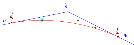
It may not be possible to design an equal tangent curve to pass through multiple design points, Figure B-22. A single curve can be fit if each of the points can be missed by a specified amount. Least squares could be applied in this case to create a best-fit curve.
 |
| Figure B-22 Multiple Design Points |
Or one of the points could be treated as the most critical and used to design a curve, Figure B-23.
 |
| Figure B-23 Critical Point Fit |
Another possible approach is to use a compound vertical curve which will be covered next.
e. Spreadsheet
An Excel spreadsheet to fit a vertical curve based on high/low point or station and elevation can be downloaded here. It uses Visual Basic for Applications script so Excel must have macros enabled when loading the sheet.