E. Traverse Adjustment
1. Adjusting a Traverse
Adjusting a traverse (also known as balancing a traverse) is used to distributed the closure error back into the angle and distance measurements.
|
Summing the latitudes and departures for the raw field traverse:
|
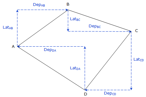 |
||
| Figure E-1 Loop Traverse Misclosure |
|||
|
On an adjusted (balanced) traverse:
|
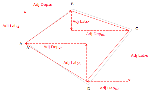 |
||
| Figure E-2 Adjusted (Balanced) Loop Traverse |

The condition for an adjusted traverse is that the adjusted Lats and Deps sum to 0.00. As with other survey adjustments, the method used to balance a traverse should reflect the expected error behavior and be repeatable. Table E-1 lists primary adjustment methods with their respective advantages and disadvantages.
| Table E-1 | |||
| Method | Premise | Advantage | Disadvantage |
| Ignore | Don't adjust anything. | Simple; repeatable | Ignores error |
| Arbitrary | Place error in one or more measurements | Simple | Not repeatable; ignores error behavior |
| Compass Rule | Assumes angles and distances are measured with equal accuracy so error is applied to each. | Simple; repeatable; compatible with contemporary measurement methods. | Treats random errors systematically |
| Transit Rule | Assumes angles are measured more accurately than distances; distances receive greater adjustment. | Simple; repeatable; compatible with older transit-tape surveys. | Treats random errors systematically; not compatible with contemporary measurement methods. |
| Crandall Method | Quasi-statistical approach. Angles are held and errors are statistically distributed into the distances. | Allows some random error modeling; repeatable. | Models only distance errors, not angle errors. |
| Least squares | Full statistical approach. | Allows full random error modeling; repeatable; can mix different accuracy and precision measurements; provides measurement uncertainties. | Most complicated method |
Most simple surveying projects use total stations which measure distances and angles with comparable quality. The Compass Rule is an appropriate adjustment method for these traverses. Although least squares would provide a "better" adjustment solution, it is generally overkill for a basic traverse. For more information on traverse adjustment by least squares see XVIII. Least Squares Lite.
We will concnetrate on the Compass Rule.
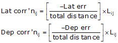
2. Compass Rule
The Compass Rule (also known as the Bowditch Rule) applies a proportion of the closure error to each line.
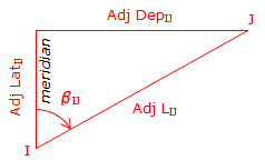
For any line IJ, Figure E-3,
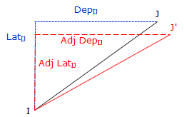 |
| Figure E-3 Adjusted Latitude and Departure |
 |
Equations E-1 and E-2 |
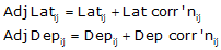 |
Equations E-3 and E-4 |
The Compass Rule distributes closure error based on the proportion of a line's length to the entire distance surveyed.
3. Adjusted Length and Direction
Regardless of the adjustment method applied, changing a line's Lat and Dep will in turn change the length and direction of the line.
 |
| Figure E-4 Adjusted Length and Direction |
The adjusted length can be computed from the Pythagorean theorem:
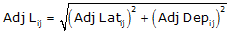 |
Equation E-5 |
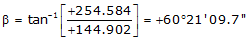
Computing direction is a two-step process: (1) Determine β, the angle from the meridian to the line (2) Convert β into a direction based on the line's quadrant.
To determine β:
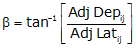 |
Equation E-6 |
β falls in the range of -90° to +90°.
The sign on β indicates the direction of turning from the meridian: (+) is clockwise, (-) is counter-clockwise. The combined signs on the adjusted Lat and Dep will identify the line's quadrant.
Figure E-5 shows the quadrant and direction computation for the various mathematic combinations of the adjusted Lat and Dep:
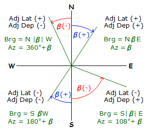 |
| Figure E-5 Converting ß to a Direction |
4. Examples
These examples are a continuation of those from the Latitudes and Departures chapter.
a. Traverse with Bearings
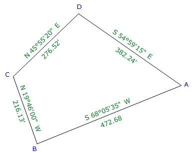 |
| Figure E-6 Bearing Traverse Example |
| Line | Bearing | Length (ft) | Lat (ft) | Dep (ft) |
| AB | S 68°05'35"W | 472.68 | -176.357 | -438.548 |
| BC | N 19°46'00"W | 216.13 | +203.395 | -73.093 |
| CD | N 45°55'20"E | 276.52 | +192.357 | +198.651 |
| DA | S 54°59'15"E | 382.24 | -219.312 | +313.065 |
| sums: | 1347.57 | +0.083 | +0.075 | |
| Distance | Lat err too far N |
Dep err too far E |
(1) Adjust the Lats and Deps
Setup Equations E-1 and E-2:
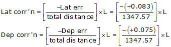
Now solve Equations E-3 and E-4 for each line:
Line AB
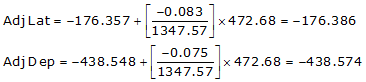
Line BC
Line CD
Line DA
Check the closure condition
| Adjusted | ||
| Line | Lat (ft) | Dep (ft) |
| AB | -176.386 | -438.574 |
| BC | +203.382 | -73.105 |
| CD | +192.340 | +198.635 |
| DE | -219.336 | +313.044 |
| sums: | 0.000 | 0.000 |
| check | check | |
A common mistake is to forget to negate Lat err and Dep err in the correction equations. If that happens, the closure condition will be twice what it originally was as the corrections were applied in the wrong direction.
(2) Compute adjusted lengths and directions
Use Equations E-5 and E-6 along with Figure E-5 to compute the new length and direction for each line.
Line AB
Adj Lat = -176.386 <- South
Adj Dep = -438.574 <- West
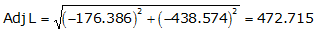
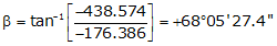
Because it's the SW quadrant, Brng =S 68°05'27.4" W.
Line BC
Adj Lat = +203.382 <- North
Adj Dep = -73.105 <- West
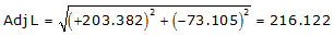
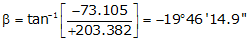
Because it's the NW quadrant, Brng = N 19°46'14.9" W
Line CD
Adj Lat = +192.340 <- North
Adj Dep = +198.635 <- East
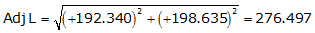
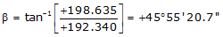
Because it's the NE quadrant, Brng = N 45°55'20.7" E
Line DA
Adj Lat = -219.336 <- South
Adj Dep = +313.044 <- East
![]()
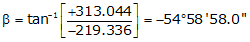
Because it's the SE quadrant, Brng = S 54°58'58.0" E
(3) Adjustment summary
| Adjusted | Adjusted | |||
| Line | Lat (ft) | Dep (ft) | Length | Bearing |
| AB | -176.386 | -438.574 | 472.715 | S 68°05'27.4" W |
| BC | +203.382 | -73.105 | 216.122 | N 19°46'14.9" W |
| CD | +192.340 | +198.635 | 276.479 | N 45°55'20.7" E |
| DE | -219.336 | +313.044 | 382.237 | S 54°58'58.0" E |
b. Traverse with Azimuths
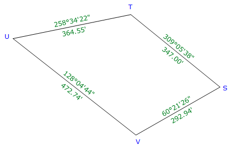 |
| Figure E-7 Azimuth Traverse Example |
| Line | Azimuth | Length (ft) | Lat (ft) | Dep (ft) |
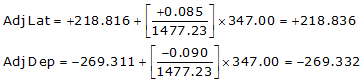
| ST | 309°05'38" | 347.00 | +218.816 | -269.311 |
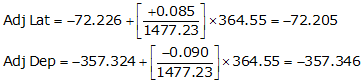
| TU | 258°34'22" | 364.55 | -72.226 | -357.324 |
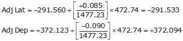
| UV | 128°04'44" | 472.74 | -291.560 | +372.123 |
| VS | 60°21'26" | 292.94 | +144.885 | +254.602 |
| sums: | 1477.23 | -0.085 | +0.090 | |
| Distance | Lat err too far S |
Dep err too far E |
(1) Adjust the Lats and Deps
Setup Equations E-1 and E-2:
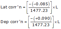
Solve Equations E-3 and E-4 for each line:
Line ST
Line TU
Line UV
Line VS
Check the closure condition
| Adjusted | ||
| Line | Lat (ft) | Dep (ft) |
| ST | +218.836 | -269.332 |
| TU | -72.205 | -357.346 |
| UV | -291.533 | +372.094 |
| VS | +144.902 | +254.584 |
| sums: | 0.000 | 0.000 |
| check | check | |
(2) Compute adjusted lengths and directions
Use Equations E-5 and E-6 along with Figure E-5 to compute the new length and direction for each line.
Line ST
Adj Lat = +218.836 <- North
Adj Dep = -269.332 <- West
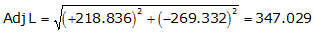
Because it's in the NW quadrant: Az = 360°00'00"+(-50°54'20.4") =309°05'39.6"
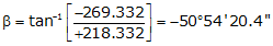
Line TU
Adj Lat = -72.205 <- South
Adj Dep = -357.346 <- West
Because it's in the SW quadrant: Az = 180°00'00"+(78°34'36.0") = 258°34'36.0"
Line UV
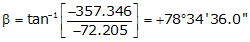
Adj Lat = -291.533 <- South
Adj Dep = +372.094 <- East
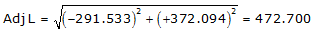
Because it's in the SE quadrant: Az = 180°00'00"+(-51°55'17.6") = 128°04'42.4"
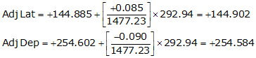
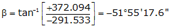
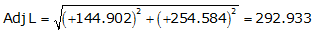
Line VS
Adj Lat = +144.902 <- North
Adj Dep = +254.584 <- East
Because it's in the NE quadrant: Az = 60°21'09.7"
(3) Adjustment summary
| Adjusted | Adjusted | |||
| Line | Lat (ft) | Dep (ft) | Length (ft) | Azimuth |
| ST | +218.836 | -269.332 | 347.029 | 309°05'39.6" |
| TU | -72.205 | -357.346 | 364.568 | 258°34'36.0" |
| UV | -291.533 | +372.094 | 472.700 | 128°04'42.4" |
| VS | +144.902 | +254.584 | 292.933 | 60°21'09.7" |
c. Crossing Loop Traverse
As long as a traverse closes back on its beginning point, it can be adjusted the same as any other loop traverse.
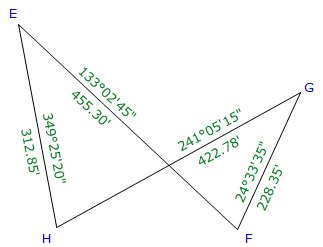 |
| Figure E-8 Crossing Loop Traverse Example |
| Line | Azimuth | Length (ft) | Lat (ft) | Dep (ft) |
| EF | 133°02'45" | 455.30 | -310.780 | +332.737 |
| FG | 24°33'35" | 228.35 | +207.691 | +94.912 |
| GH | 241°05'15" | 422.78 | -204.403 | -370.084 |
| HE | 349°25'20" | 312.85 | +307.534 | -57.430 |
| sums: | 1419.28 | +0.042 | +0.135 | |
| Dist | Lat err too far N |
Dep err too far E |
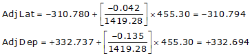
(1) Adjust and recompute each line.
Setup Equations E-1 and E-2:
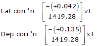
Solve Equations E-3 and E-4 for each line:
Line EF
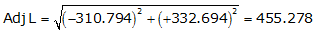
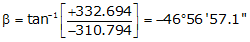
Because it's in the SE quadrant: Az = 180°00'00"+(-46°56'57.1") = 133°03'02.9"
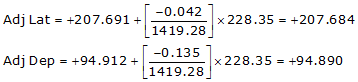
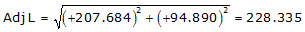
Line FG
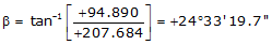
Because it's in the NE quadrant: Az = 24°33'19.7"
Line GH
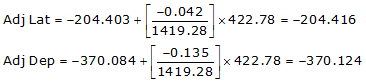
Because it's in the SW quadrant: Az = 180°00'00"+(61°05'18.8") =241°05'18.8"
Line HE
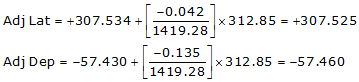

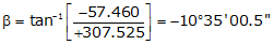
Because it's in the NW quadrant: Az = 360°00'00"+(-10°35'00.5") = 349°24'59.5"
(2) Adjustment summary
| Adjusted | Adjusted | |||
| Line | Lat (ft) | Dep (ft) | Length (ft) | Azimuth |
| EF | -310.794 | +332.694 | 455.278 | 133°03'02.9" |
| FG | +207.684 | +94.890 | 228.335 | 24°33'19.7" |
| GH | -204.416 | -370.124 | 422.821 | 241°05'18.8" |
| HE | +307.525 | -57.460 | 312.847 | 349°24'59.5' |
| sums: | -0.001 | 0.000 | ||
| check (rounding) | check | |||
5. Summary
A traverse is adjusted, or balanced, to distribute remaining random errors back into the measurements. There are a number of ways to accomplish this differing in how the errors are modeled and computation complexity. The Compass Rule demonstrated here works well for simple traverses having minimal redundant measurements. The examples thus far are closed loop traverses. Chapter H. Closed Link Traverse shows how to perform traverse computations, including adjustments, on closed link traverses.
The Compass and Transit Rules and Crandall Method are compared using a numeric example in Chapter K. Comparison of Adjustment Methods. Traverse Adjustment, an Excel workbook for the three methods, is in the Software area. As traverses become more complex with additional measurements added, particularly with mixed quality, a least squares adjustment is the best strategy to employ. This concept is discussed in greater detail in XV. Least Squares Lite topic.