J. Coordinate Transformation
1. A typical scenario
Surveyor Jones traversing Lot 3 in a subdivision assumes the coordinates of one property corner and the direction of a line, Figure J-1.
|
|
|
Figure J-1 |
Later, Surveyor Davis is hired to map Lot 4 next door to the east. He assumes his own coordinates and line direction, Figure J-2.
|
|
|
Figure J-2 |
Both surveyors have good closure and compute coordinates for their lot corners.
Today, you are hired to do a survey in the vicinity of the two lots. Realizing that Jones' line CD and Davis' line TU are the same line, you decide to plot both their surveys in CAD (Computer Assisted Drawing). The result? Figure J-3.
|
|
|
Figure J-3 |
Something doesn't look right - the two lots are supposed to be next to each other.
What happened?
The two surveys are in separate coordinate systems. Since each surveyor assumed his own starting coordinate and direction independent of each other, they have different coordinate origins and meridian (North) direction. To resolve this problem we need to move Lot 3 into Lot 4's system or Lot 4 into Lot 3's system, Figure J-4, We also have the option of moving both to a third system.
|
|
|
Figure J-4 |
There are a few ways to do this. We could:
- reduce Davis' survey data using Jones' coordinate system
- perform a coordinate transformation.
Regardless of the method, we must know something about how both surveyors' systems are related to each other.
2. Transforming coordinates
A coordinate transformation changes point positions from one coordinate system to another. It does not require the original measurements used to create the coordinates. Figure J-5 illustrates a situation similar to combining Jones' and Davis' surveys: the same two physical points (A abd B) have two different mathematical positions.
|
|
|
Figure J-5 |
The two coordinate systems are To and From. The To system is final coordinate system in which we'd like all positions expressed. Points AT and BT are the points correctly located in the To system. Points AF and BF are the same points but in a the From system. Points CF and DF are also in the From system and we would like to know their coordinates in the To system.
A transformation consists of three elements
- Scaling
- Rotation
- Translation
We'll discuss the elements in the order shown. To differentiate between the systems we'll used X, Y coordinates for the From system and N, E for the To.
3. Transformation elements
b. Scaling
Scaling is used to increase or decrease distances between the points in order to make them fit in the new system. The distances may be off due to:
- random errors
- systematic errors
- unit conversion (eg, meters to feet)
- ground to grid distortion (in larger regional systems)
- combinations of the above.
To scale the transformation, we need the length of the same line in both systems, Figure J-16. The length can be from direct measurement (and subsequent adjustment) or by inversing between the coordinates of two common points.
|
|
|
Figure J-6 |
The scale is a ratio between the To and From system line lengths, Equation J-1.
| Equation J-1 | ||
|
LT |
To length |
|
Scaling isn't always necessary depending on the circumstances and allowable error. For example, if a maximum error of 1/20,000 is acceptable, then a scale in the range of 1±1/20,000 (0.99995 to 1.00005) can be treated as 1.00000 and this step skipped.
When accounting for scale there are three approaches:
- Unitary - Maintains a 1:1 relationship between the two coordinate systems.
- Uniform - Enforces the same consistent scale (other than 1) in all directions. Only a single scale is computed for the entire transformation.
Both Unitary and Uniform approaches are referred to as a Conformal Transformation because true shapes are maintained. - Differential - Scale in the North-South direction differs from scale in the East-West direction. Two different scales (SN and SE) are computed for the transformation. This is referred to as an Affine Transformation.
Scale is radially applied from the To system's origin. Once applied another set of updated From coordinates, subscripted 1, are created, Figure J-7.
|
|
|
Figure J-7 |
b. Rotation
The From coordinates must be rotated to make its directions coincide with those of the To system. To determine the rotation angle we need the direction of a common line in both systems. In Figure J-8, we need to make the direction of line AFBF the same as the direction of line ATBT.
|
|
|
Figure J-8 |
Beacuse a line doesn't physically rotate, we need to make the North meridian of the From system parallel with To's. For example, line JK has an assumed azimuth of 270°00'00"; the same line has a true azimuth pf 245°00'00". The line is the same in both systems, only the directions of North differ, Figure J-9.
|
|
|
Figure J-9 |
The rotation angle, ρ, is the amount the Assumed North must be rotated to coincide with the True North. In this case, it must be rotated clockwise (to the right) by 270°00'00"-245°00'00" = +25°00'00".
If the Assumed azimuth is 215°00'00" and True azimuth is 245°00'00", Figure J-10, then Assumed North must be rotated counter-clockwise (to the left) which means it must be a negative angle: 215°00'00"-245°00'00" = -30°00'00".
|
|
|
Figure J-10 |
The rotation angle, ρ, is the From direction minus the To direction, Equation J-2.
| Equation J-2 | ||
|
DirT |
To direction | |
|
DirF |
From direction | |
If using two control points, inversing between them in both systems will provide the requisite directions.
The rotation point is the origin of the To coordinate system. The effect of rotating the From meridian creates another updated From coordinate set, sub-scripted 2 in Figure J-11.
|
|
|
Figure J-11 |
c. Translation
The final element consists of two translations: shift positions in the North-South and East-West directions. These are the differences at one point between its To and updated From coordinates, Figure J-12.
|
|
|
Figure J-12 |
Translations are computed from a control point known in both systems. Because the rotation and scale have already been applied, they must be incorporated to determine the translations. The translations are Equations J-3 and J-4 in terms of the original From system.
|
|
Equation J-3 |
|
|
Equation J-4 |
These two final elements complete the transformation, Figure J-13.
|
|
|
Figure J-13 |
e. Transformation Equations
Once the parameters are determined, they are assembled to create the transformation equations, J-5 and J-6, which are used to move other points to the To system, Figure J-14.
|
|
|
| Equation J-6 | |
|
|
|
|
|
Figure J-14 |
f. CAD equivalent
Consider how you would solve this problem in Figure J-3 using CAD. You would use CAD Move, Rotate, and Scale operations, Figure J-15, to put Lot 4 in Lot 3's system. What you've done is apply a coordinate transformation graphically.
|
|
|
Figure J-15 |
g. Number of parameters
A coordinate transformation is sometimes referred to as either a three-, four- or five-parameter transformation. The difference between the number of parameters is how scale is applied. Either way, a certain amount of data (control) is needed in both systems. Each parameter is an unknown which must be solved. This will dictate the minimum amount and type of control that is needed.
| Table J-1 | |||
| Transformation type | Three parameter (Conformal) |
Four Parameter (Conformal) |
Five-Parameter (Affine) |
| Parameters | TN TE ρ |
TN TE ρ S |
TN TE ρ SN SE |
| Scale | Scale = 1 | Single scale in all directions | N/S and E/W scales can differ |
| Control needed in both systems | One point's coordinates, one line's directions |
One point's coordinates, one line's direction, one line's distance |
One point's coordinates, one line's directions, two line's distances |
| or | or | or | |
| two points | two points | two points & one line's directions | |
| or | |||
| three points | |||
These are generally the minimal amounts of control needed to uniquely determine the transformation parameters. For example, a four-parameter transformation has four unknowns. Two control points contribute four knowns: two coordinate pairs. Having only a single control point won't allow you to compute the transformation parameters. At best, you can translate the From coordinates, but there isn't sufficient information to determine a rotation or scale.
Using just the minimum control means errors in the control will be undiscovered and become part of the parameters affecting all points transformed. Additional control data can be used for math checks. Due to the presence of random errors, different combinations of control will result in slightly different transformation parameters. To get a better model which propagates the error into the final positions, all control should be incorporated in a least squares transformation. Creating such a model manually is time consuming so we will not address least squares transformations here. Many surveying software packages usually include an optional least squares transformation.
We will concentrate on the four-parameter model as it works well for most ground-based survey applications. Including a uniform scale absorbs smaller random errors satisfactorily as long as good control is used.
4. Variations
While a full coordinate transformation includes rotation, scaling, and translation, there are situations where only one or two of the elements are necessary.
a. Rotation only
A rotation-only transformation is used to convert directions from one meridian reference to another. An example is converting magnetic to true directions.
Traverse line directions in Figure J-16 are referenced to Magnetic North.
|
|
|
Figure J-16 |
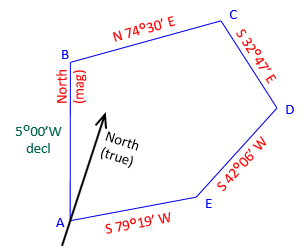
To obtain True bearings, each bearing must change numerically by 5°00' to the West to compensate for the declination. Figure J-17 Shows Magnetic and True meridians at each point.
|
|
|
Figure J-17 |
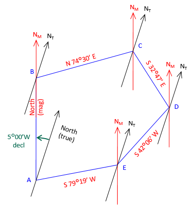
The True bearing of line AB is N 5°00' W; line BC is N69°30'E; line CD is S 37°47'E; ...
b. Translation only
When dealing with regional coordinate systems, the corners of a small survey may have large coordinates, Figure J-18. To work with smaller coordinates, the surveyor may subtract a one constant from all the North coordinates and another constant from the East coordinates.
|
|
|
Figure J-18 |
For traverse in Figure J-18, we could subtract 384,000.00 from the North coordinates and 2,307,000.00 from the East coordinates. The result would be Figure J-19.
|
|
|
Figure J-19 |
This effectively creates a local origin shown in Figure J-20 with trranslation parameters.
|
|
|
Figure J-20 |
Coordinate differences are still the same since each coordinate pair has been changed the same amount. Inverse and area computations are similarly unaffected outside the fact that the magnitude of the computations are somewhat simplified.
c. Translation and rotation
A typical field situation could be collecting data referenced to a base line without first knowing the base line's location. The data is relative to the base line so later fixing the base line fixes the data.
A field crew sets up on one control station and uses another as a backsight for a topo survey. Not knowing coordinates of either point they assume the coordinates of A, their total station instrument (TSI) location, and direction of the backsight line. From there they collect and reduce their topo data.
Later they are able to obtain point A's coordinates and the correct direction to point B. Figure J-21 shows what happened when they incorporate the control with their field data .
|
|
|
Figure J-21 |
Using this information, they are able to translate and rotate the topo data to its correct location, Figure J-22.
|
|
|
Figure J-22 |
5. Numeric Example
A crew surveyed the exterior of a parcel, Figure J-23. They assumed the coordinates of the southernmost corner (1001) and used the record bearing for the southwesterly line (1001-1002)
|
Figure J-23 |
|||||||||||||||
|
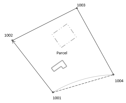
Later, a second survey crew was sent out to locate the existing drainfield. They did not have the first crew's coordinates so they occupied the northernmost corner (NE), for which they assumed coordinates, and backsighted the westernmost corner (NW), for which they assumed a direction. They then shot the drainfield corners. As a check, they also shot the distance from NE to NW. Figure 24 is a summary of their survey.
|
Figure J-24 |
Assumed dir NE-NW: N 90°00'00" W |
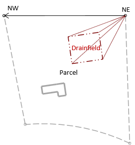
The data was combined in a CAD drawing with the result shown in Figure J-25.
|
|
|
Figure J-25 |
Using the boundary survey as the reference system, translate the drainfield data.
a. Determine transformation parameters
Step (1) Scale
Length of line NE-NW is 476.41', line 1003-1002 is 476.37'.
From Equation J-1:
![]()
This represents a distortion of 1/(1-0.999916) = 1/11,900. If this is within tolerance, then the scale factor can be ignored. We will apply it in this example.
Step (1) Rotation angle
Line NE-NW coincides with line 1003-1002; Convert the bearings to azimuths and compute the rotation angle.
| Line NE-NW | |
| Line 1003-1002 | |
|
Using Equation J-2
|
|
 -
-Step (3) Translations
Use the coordinates of points 1003 and NE in Equations J-3 and J-4 to determine the translations.
![]()
![]()
Step (4) Math check
For a parameters math check, convert NW to see if it matches the coordinates of 1002.
In the From system, NW's coordinates are:

Transform and check:
![]()
![]()
Yuo, it checks.
b. Using Equations J-5 and J-6 transform the drainfield corners: 501-504
Point 501
![]()
![]()
Point 502
![]()
![]()
Point 503
![]()
![]()
Point 504
![]()
![]()
6. Two-Dimensions vs Three-Dimensions
While the discussion here is limited to horizontal (two dimensional) coordinate systems, it is relatively easy to extend this into the third dimension by incorporating elevations or Z coordinates. An additional translation parameter would be needed for the elevation component, TElev.
The rotation angle, ρ, for a two dimensional transformation is a horizontal angle rotated about the vertical, or Z, axis. In a three dimensional transformation there would three rotation angles, one about each axis. Figure J-25 shows X-Y-Z as the From system and E-N-Elev as the To system. There are three rotations and three translations. How about scale?
|
|
|
Figure J-25 |
Scale could again be Unitary, Uniform, or Differential. In the latter case, there would be three scale factors.
The total number of parameters in a three dimensional transformation could be:
- Six: Three translations, three rotations, 1:1 scale
- Seven: Three translations, three rotations, uniform scale
- Eight: Three translations, three rotations, one scale for horizontal, one scale for vertical
- Nine: Three translations, three rotations, three scales
The eight-parameter transformation could be used where there is a quality difference between horizontal and vertical positions in one system or the other.
7. Summary
A coordinate transformation gives a the surveyor the ability to move position information from one coordinate reference system to another. The amount of error introduced into the new positions is a function of the mathematical model used to perform the transformation and the control quality. Examples, as shown in this section, which use minimal control to determine unique model parameters have the effect of spreading a mistake or systematic error through all the data points. Additional control provides some math checking although it will not be perfect due to the presence of random errors.
There are many coordinate transformation models beyond those discussed here. The relationship between the From and To systems can be complicated and extremely variable even over small areas requiring more complex modeling than simple Conformal or Affine transformations. Unless there is an exact mathematical relationship between the From and To systems, a transformation will introduce some degree of positional error. The error can be minimized, but not eliminated, by using complex models, keeping the area small, and ensuring redundant quality control is used. The best way to determine transformation parameters is by least squares which not only better models errors, but propagates them into the new positions. Complex models and least squares application are beyond the scope of this topic. Surveying or mapping software users are encouraged to consult their documentation to see what options are available. The National Geodetic Survey (NGS) has some transformation related publications and software tools on its website (https://www.ngs.noaa.gov/).
A simple 2D Conformal Transformation Excel workbook is in Software | Excel Workbooks. A more comprehensive Windows program, TransPack, performs Conformal, Affine, and Projective transformations using least squares. It can transform single points or point files. The software is described and available for download at Software | Coordinate Transformations.