Chapter D. Projection Surfaces

This chapter is a simplified discussion of map projections. It covers systems typically used in surveying applications which are a small subset of the larger map making science. For those interested in more detail, "Map Projections - A Working Manual", USGS Prof Paper 1395 by John P. Snyder is an excellent technical resource. It thoroughly covers map projections and includes their equations with computational examples. At the time of this writing (11/2021) It was available as a free download at https://pubs.usgs.gov/pp/1395/report.pdf.  

1.The Ellipsoid

The Earth is more complex than tomatoes or oranges and not a good mathematical model from which to project points. In the Horizontal Datums topic we saw how an ellipsoid, Figure D-1, was developed as a mathematical model of the Earth.

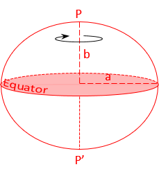Figure D-1 Ellipsoid

a, b are the semi-major and -minor axes, respectively

Heights, Figure D-2, allow us to project points from the physical earth to the ellipsoid.
 

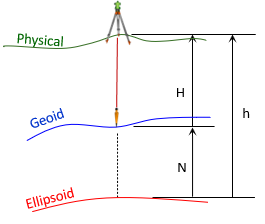Figure D-2 Heights

Where

• H: orthometric height
• N: geoid height
• h: geodetic height

Once points are on the ellipsoid, they can be mathematically projected to a developable surface from which a 2D grid can be constructed.

2. Projections

a. Developable Surfaces

A developable surface is one that is either flat or can be rolled out flat without distorting it. Points are projected from the ellipsoid to the surface. Because the surface is mathematically connected to the ellipsoid, distortions can be controlled by limiting the area projected or compensated by computation.

There are three primary developable surfaces, each has advantages and disadvantages for grid system construction.

(1) Plane

A plane is the simplest because it is already flat. North and East axes are added, Figure D-3, creating a coordinate system .

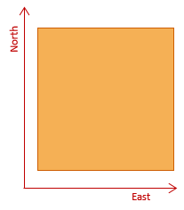Figure D-3 Plane Surface

(2) Cone

A cone can be cut from bottom to tip, rolled out flat, and a coordinate system added, Figure D-5.

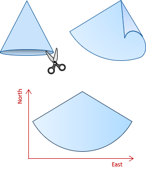Figure D-5 Conic Surface

(3) Cylinder

A cylinder can be cut axially, rolled out flat, and a coordinate system added, Figure D-4.

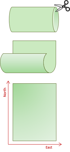Figure D-4 Cylindric Surface

b. Projection Type

Ellipsoid points can be mathematically projected to a developable surface many different ways. Although distortions are unavoidable, certain spatial conditions can be favored at the expense of others. For example, two common projection conditions are:

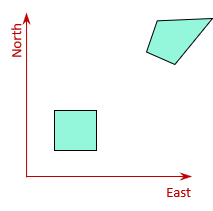
• Equal-Area - Area is consistent at different locations while distances and angles can change. A square in one part the projection will have the same area when moved to a different location although its shape will be distorted, Figure D-5.

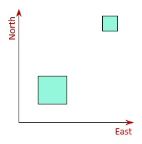
• Conformal - Angular relationships around a point are maintained. A square in one part of a projection will still be a square at another location although its size will be different, Figure D-6. These are also called orthomorphic projections.

Figure D-5 Equal-Area Projection	Figure D-6 Conformal Projection

Regional coordinate systems for large scale applications and used by surveyors are generally based on conformal projections.

3. A matter of Scale

a. Distance Distortion

Distances are distorted when projected from the ellipsoid to a developable surface. The distortion can be stated as a ratio or a scale.

• A ratio is a unit distortion per a specific distance. A ratio of 1:5,000 or 1/5,000 means a 5,000 ft distance will be distorted by ± 1 ft, a 10,000 ft by ±2 ft, etc.  A 1/10,000 distortion is less than 1/5,000.
• A scale is a ration converted to a multiplier. Since the distortion can be ±, its scale is a range. 1/10,000 as a scale is a range between (1-1/10,000) and (1+1/10,000) which is 0.9999 to 1.0001.

Scale is systematic and can be compensated mathematically. However, for many applications, grid and geodetic distances can be considered the same below some maximum scale. This can reduce computations substantially.

Surface fit and area extent affect how distance distortion behaves.

b. Surface Fit

A developable surface can be either tangent or secant to the ellipsoid.

• A tangent fit touches the ellipsoid at a single point (plane) or along a line (cylinder and cone).
• A secant fit cuts through the ellipsoid along an ellipse (plane) or two parallel lines (cylinder and cone).

Figure D-7 shows an ellipsoid section with evenly spaced points.

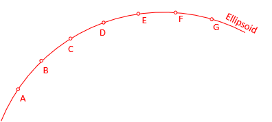Figure D-7 Points on the Ellipsoid

Except where it intersects the ellipsoid, a tangent surface is everywhere outside the ellipsoid, Figure D-8.

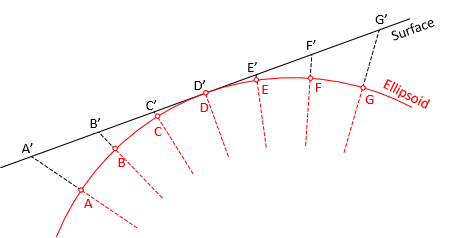Figure D-8 Tangent Surface Fit

Points are projected to the surface, displacing them outward from the tangent location. The further away, the greater the displacement. Distances increase accordingly: D'E' < E'F' < F'G'. Scale at the tangent location is exactly 1 and gets larger further away. Scale is never less than 1 on a tangent surface.

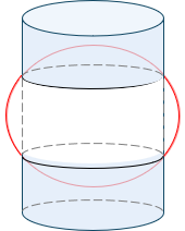
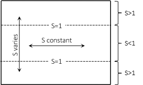
A secant surface is part inside and part outside the ellipsoid, Figure D-9.

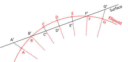Figure D-9 Secant Surface Fit

Ellipsoid points projected inward to the surface shorten the distances in between; Scale<1.
Ellipsoid points projected outward to the surface lengthen the distances in between; Scale>1.
Scale is 1 at the intersection where there is no displacement.

Because a tangent surface's scale is always equal to or greater than 1, its use is generally limited to a smaller area. A secant surface can cover a greater area since its scale varies between less than and greater than 1. Most commonly used regional grid systems are based on secant projections.

4. Secant Projections

a. Plane

Depending on its orientation, a secant tangent intersects the ellipsoid along a circle or ellipse, Figure D-10.

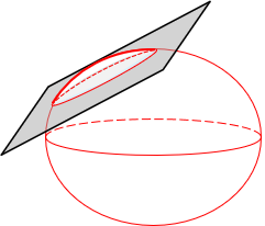Figure D-10 Secant Plane

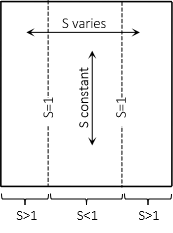
Inside the intersection scale is less than 1, outside greater than 1; along the intersection it is 1.
On the plane, Figure D-11, scale varies radially perpendicular to the intersection path, constant parallel with it.

Figure D-11 Secant Plane Scale

Movement in any direction other than parallel with the intersection will cause scale variations. Line lengths don't change uniformly between the ellipsoid and grid. This limits plane projections to small areas or where larger variable distortions are tolerable. A plane projection is generally too restrictive for a regional survey-quality coordinate system.

b. Cone

A secant cone is oriented so its axis coincides with the polar axis, Figure D-12.

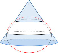Figure D-12 Cone Orientation

It intersects the ellipsoid along two lines of latitude. When rolled out flat the two intersecting lines are arcs centered on the cone's apex. Because they are lines of latitude, Figure D-13, they run east-west and are called standard parallels. Geodetic meridians converge to the cone apex.

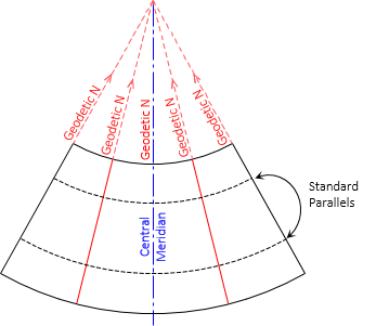Figure D-13 Conic Geodetic Meridians and Parallels

Scale along standard parallels is 1; between them it is less than 1, outside greater than 1. Scale is constant along parallels of latitude and varies along geodetic meridians, Figure D-14.

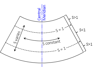Figure D-14 Conic Scale

Conic projections are used for areas longer east-west than north-south. The most commonly used is the Lambert Conic projection developed by mathematician Johann Heinrich Lambert in 1792.

c. Cylinder

(1) Mercator Cylindric Projection

One of the first universally adopted cylindric projections was developed in 1569 by Gerardus Mercator. His projection was oriented with the cylinder's axis parallel with the Earth's rotational axis. The Mercator projection intersects the ellipsoid along two lines of latitude, one on each side of the equator, Figure D-14.

Figure D-14 Mercator Cylindric Projection

The projection was widely used for ship navigation, A ship sailing along a constant azimuth travels a curved path on the earth. On a Mercator projection, the ship's course is a straight line making navigation easier.

When rolled out flat the two intersection lines project as east-west lines, also called Standard Parallels. Instead of converging, geodetic meridians project parallel, Figure D-15

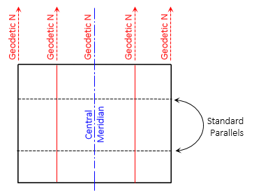Figure D-15 Cylindric Geodetic Meridians and Parallels

Scale along standard parallels is 1; between them it is less than 1, outside greater than 1. Scale is constant east-west and varies north-south along meridians. Figure D-16.

Figure D-16 Mercator Cylindric Scale

Because geodetic meridians project parallel, object shapes can be substantially distorted. Minimizing scale requires keeping the Standard Parallels close to the equator. Distortion is least near the equator and gets much larger toward the poles.

A example Mercator cylindric projection is shown in Figure D-17.

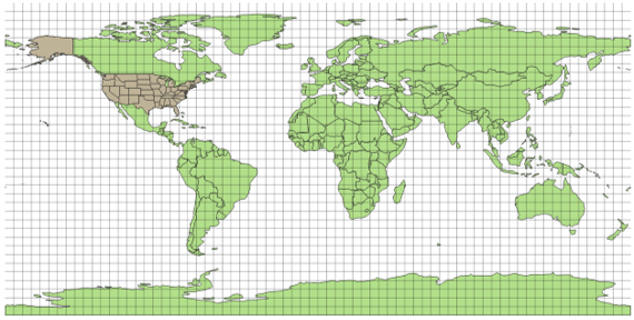Figure D-17 Worldwide Mercator Cylindric Projection

Latitudinal lines and meridians are straight and equally spaced. Country shapes look "correct" near the equator. Moving north and south, shapes are "stretched" east-west because meridians do not converge. At the latitude of the United States,distortions exceed acceptable values for large scale mapping. A traditional Mercator cylindric projection is too limited for regional surveying coordinate systems.

(2) Transverse Mercator Cylindric Projection

Johann Heinrich Lambert (yup, the Cone-head) developed a version of Mercator's cylinder turned on its side, the Transverse Mercator cylindric projection, Figure D-18.

Figure D-18 Transverse Mercator Cylindric Projection

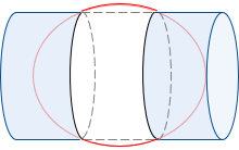
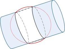
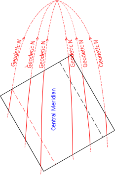
A transverse cylindric projection offers greater design flexibility and distortion control. It intersects the ellipsoid along two parallel ellipses. These ellipses are parallel with, and equidistant from, the central meridian. When rolled out flat, the two intersection lines project as straight lines, Figure D-19.

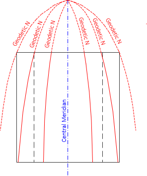Figure D-19 Transverse Cylindric Meridians

Geodetic meridians converge and, except for the central meridian, are curved. The degree of curvature depends on the latitude and size of the area.

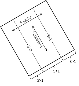
Scale is 1 along the intersection lines; it is less than 1 between and greater than 1 outside the intersection lines, Figure D-20.

Figure D-20 Transverse Cylindric Scale

Scale is generally constant north to south and varies east to west. Because of this, a transverse cylindric projection is used for regions longer north-south than east-west.

(3) Oblique Mercator Cylindric Projection

A region's long axis can be oriented other than north-south or east-west. Conic and traditional or transverse cylindric projections may not fit the area well. In cases like this, an oblique cylindric projection can be used. An oblique cylinder is rotated so its axis direction is neither polar or equatorial, Figure D-21.

Figure D-21 Oblique Secant Cylinder

The oblique cylinder intersects the ellipsoid along two ellipses. When the cylinder is rolled out flat, the intersections project as straight lines. Geodetic meridian behavior is the same as a transverse cylindric project but rotated to the projection surface, Figure D-22.

Figure D-22   Oblique Cylindric Meridians

Scale along the intersecting lines is 1; between it is less than 1, outside greater. Scale is constant in the rotated direction and varies perpendicular to it, Figure D-23.

Figure D-23 Oblique Cylindric Scale