6. Example Adjustment
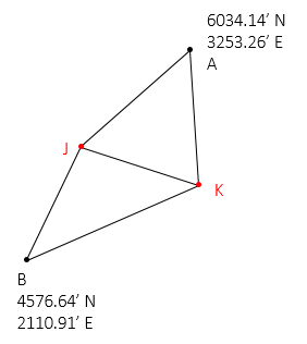
Given the network and data in Figure F-5, determine:
- adjusted coordinates of points J and K.
- their standard errors
- adjusted observations
- their standard errors
 |
 |
| Figure F-5 Combined Observations |
There are seven observations and four unknowns: NJ, EJ, NK, EK. The network has 7-4 = 3 DF.
a. Matrix structures
Matrix structures are:


b. Initial approximations for points K and J
The computations are summarized and results shown:
- Distance and direction for line BA by inverse
- Solve angle ABK using Law of Cosines: 28°28'09"
- Compute direction of BK using direction BA and angle ABK: 66°33'27"
- Use direction BK and 1309.94' to compute coordinates of K: 5097.77' N, 3312.73' E
- Solve angle JBA using Law of Cosines: 11°56'48"
- Compute direction of BJ using direction BA and angle JBA: 26°08'30"
- Use direction BJ and 871.35' to compute coordinates of J: 5358.86' N, 2494.82' E
c. Compute weight matrix


d. Distances
The distances are computed from the fixed coordinates of A and B and the initial approximations of J and K.

e. Build [C] and [K] matrices
Note: it is extremely important to minimize rounding errors by carrying enough digits in computations. Not doing so can either increase the number of iterations needed for a solution or could cause the solution to diverge.
(1) Distance observations
Obs 1: Line KB

Obs 2: Line KJ

Obs 3: Line KA

Obs 4: Line JA

Obs 5: Line JB

(2) Angle observations
Obs 6: Angle BKJ


Obs 7: Angle JKA


(3) Assemble [C] and [K] matrices


f. Solve U=[Q] x [CTWK]
Rather than detail the complete solution process, the matrices and partial products are shown for each iteration. Just remeber that after each iteration, the entire [C] and [K] matrices must be recomputed.
(1) First Iteration


The corrections aren't small enough so update the coordinates and repeat solution.
Updated coordinates:

Repeat as corrections are not small enough.
(2) Second Iteration
Using the updated coordinates, go back to Step d, recompute distances and matrices, and solve for [U].


The corrections still aren't small enough so update the coordinates and repeat solution.
Updated coordinates:

(3) Third Iteration


Corrections are acceptably small enough. Update coordinates one last time.

g. Compute statistics
(1) Compute So and adjusted point uncertainties
Using last [C], [K] and [U] matricies, determine residuals from [V] = [C] x [U] - [K]
Use [V] and [W] to compute So , then So and [Q] to compute standard deviations of the adjusted coordinates.
 |
 |
(2) Adjusted observations
Add residuals to the original observations

Compute standard errors for the adjusted observations. Example comps are shown for distance KB and angle BKJ.
Obs 1: distance KB
Use first row of [C] and first column of [CT].

Obs 6: Angle BKJ
Use sixth row of [C] and sixth column of [CT].

Remaining standard errors are included in the following section.
h. Adjustment Summary
Degrees of freedom: DF = 7-4 = 3
Std Dev Unit Wt: So = ±2.136'
| Point | North | East | SN | SE |
| J | 5359.086' | 2494.852' | ±0.126 | ±0.210 |
| K | 5097.253' | 3313.197' | ±0.167 | ±0.076 |
| Adj Obs | S | |
| Dist KB | 1310.671' | ±0.037' |
| Dist KJ | 858.663' | ± 0.023' |
| Dist KA | 938.422' | ± 0.033' |
| Dis JA | 1019.338' | ± 0.023' |
| Dist JB | 866.611' | ± 0.022' |
| Ang BKJ | 40°47'23.4" | ±09.2" |
| Ang JKA | 68°56'54.8" | ±13.0" |