F. Nonlinear Measurements
1. Introduction
Recall that non-linear equations solution requires an iterative approach after applying the Taylor Series. In an LS application, this means initial approximations are used to formulate the [C] and [K] matrices and the [U] solution matrix has corrections for the approximations.The [C] and [K] matrices are updated and a new set of corrections determined. This repetitive process continues until the corrections are small enough to be acceptable.
The elevation observation equation, being single dimension, is linear so a leveling circuit does not require an iterative solution. A horizontal network uses distance and angles to determine two dimensional point positions. The relationship between measurements and positions is based on higher math including trigonometric functions which are not linear.
A horizontal network can be adjusted by coordinate variation. Beginning with a mathematical equation relating a measurement type to coordinates, a Taylor Series is applied to create an observation equation. Initial coordinate approximations of the unknown points are used with the observation equations for the LS adjustment to generate coordinate corrections. These are applied and the adjustment repeated until the corrections fall below a threshold. The final results are coordinates which can be used, if desired, to solve adjusted distances, azimuths, and angles.
This chapter covers three primary horizontal measurement types: distance, azimuth, and angle. Observation equations are developed to help understand the iterative nature of a horizontal adjustment. An example simple network shows how the observation equations are used in the adjustment process. Be forewarned: manually adjusting a horizontal network involves a lot of computations. Not only can it be tedious, but math errors can be easily made.
What you should get out of this chapter is that there is a lot of math involved (including calculus) in a simple horizontal network adjustment. Increasing the degrees of freedom substantially impacts the calculations which must be performed. Understanding why an iterative appraoch is necessary to adjuist the network is equally important.
2. Distance
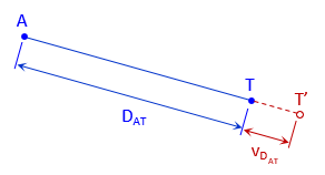 |
| Figure F-1 Distance Observation |
Equation F-1 is the distance bertween two points in terms of their coordinates.
| Equation F-1 | |
|
NA, EA: At point coordinates |
|
To apply a Taylor Series, patial derivatives of Equation F-1 are taken with respect to each coordinate of both points. The partial derivative for NA is:

Similarly, the remaining partial derivatives are:

Equation F-2 is the distance observation equation, evaluated at initial coordinate approximations.
 |
Equation F-2 | ||
| Equation F-3 | |||
3. Azimuth
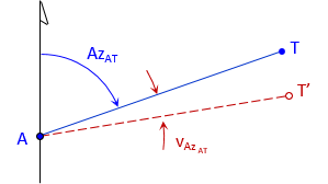 |
| Figure F-2 Azimuth Observation |
Equation F-4 is the angle of a line from the meridian in terms of a its coordinates.
 |
Equation F-4 |
|
A: At point |
|
The angle from the meridian can be to the right (+) or to left (-) depending on the coordinate differences signs. This places the angle in one of the four quadrants, Figure F-3.
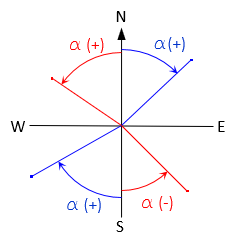 |
| Figure F-3 Angle from Meridian |
The value of QAT, added to the angle to obtain the azimuth, depends on the quadrant. Table F-1 shows the sign of α, its quadrant and QAT value.
| Table F-1 Azimuth for a Line ij by Quadrant |
 |
Partial derivatives of Equation F-4 are taken with respect to each coordinate of both points. The partial derivative for NF is:

Remaining partial derivatives are:

Equation F-5 is the azimuth observation equation, evaluated at initial coordinate approximations.
 |
Equation F-5 | |
| Equation F-6 | ||
4. Horizontal Angle
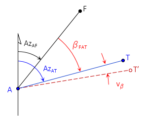 |
 |
| Figure F-4 Horizontal Angle Observation Examples |
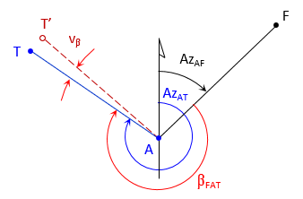
Equation F-7 is the horizontal angle observation equation in terms of point coordinates.
 |
Equation F-7 |
|
A: At point |
The horizontal angle is to the right and is the difference between azimuths from the At point (instrument location) to the To point (foresight) and From point (basksight). Equation F-7 is a combination of two Equations F-4: one for the foresight line, the other for the backsight.
Partial derivatives of Equation F-7 are taken with respect to each coordinate of all three points. The partial derivative for NA is:

Remaining partial derivatives are:

Equation F-8 is the horizontal angle observation equation, evaluated at initial coordinate approximations.
 |
Equation F-8 | ||
| Equation F-9 | |||
5. Dimensions and Units
a. Angles
When horizontal angles or directions are included in an adjustment, units must be taken into consideration. Distances may be in feet, chains, or meters. Degreee-minute-second (DMS) units are commonly used for angles and directions.
[K] matrix angle and direction elements are computed from measured angles and point coordinates. They are usually small and expressed in seconds. [C] matrix angle elements are in radians because they come from partial derivatives of the tangent trigonometric function.
The [C] and [K] matrices are used to determine the [U] and [V] matrices. To avoid mixed angular units, either the [C] matrix angle elements must be converted to seconds or the [K] matrix's to radians. For easier residual terms and standard error interpretation, [C] elements are converted to seconds multiplying each angular term by 206,265 sec/radians.
b. Mixed Measurements
Horizontal network adjustment generally includes a mix of distances, angles, and directions. Dimensions of [C] and [K] matrix elements depend on the observation equations used. If [C] and [K] dimensions are mixed, some of the elements in the [U] matrix won't be correct: some may be feet, others could be seconds-feet, which doesn't make sense. To obtain correct dimensions and units, weights must be applied to the adjustment.
As discussed in Chapter E a measurement's weight is the reciprocal of its standard error squared, 1/(SEi2). This places the measurement's squared dimension in the denominator so units cancel correctly in the [CTWC] and [CTWK] matrix products. This makes all [U] matrix elements linear.
If measurement standard errors are unknown, reasonable estimates should be used to ensure dimensions cancel correctly. Otherwise results may not be correct or the adjustment may not converge to a solution.
6. Example Adjustment
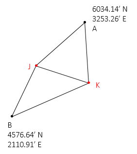
Given the network and data in Figure F-5, determine:
- adjusted coordinates of points J and K.
- their standard errors
- adjusted observations
- their standard errors
 |
 |
| Figure F-5 Combined Observations |
There are seven observations and four unknowns: NJ, EJ, NK, EK. The network has 7-4 = 3 DF.
a. Matrix structures
Matrix structures are:


b. Initial approximations for points K and J
The computations are summarized and results shown:
- Distance and direction for line BA by inverse
- Solve angle ABK using Law of Cosines: 28°28'09"
- Compute direction of BK using direction BA and angle ABK: 66°33'27"
- Use direction BK and 1309.94' to compute coordinates of K: 5097.77' N, 3312.73' E
- Solve angle JBA using Law of Cosines: 11°56'48"
- Compute direction of BJ using direction BA and angle JBA: 26°08'30"
- Use direction BJ and 871.35' to compute coordinates of J: 5358.86' N, 2494.82' E
c. Compute weight matrix


d. Distances
The distances are computed from the fixed coordinates of A and B and the initial approximations of J and K.

e. Build [C] and [K] matrices
Note: it is extremely important to minimize rounding errors by carrying enough digits in computations. Not doing so can either increase the number of iterations needed for a solution or could cause the solution to diverge.
(1) Distance observations
Obs 1: Line KB

Obs 2: Line KJ

Obs 3: Line KA

Obs 4: Line JA

Obs 5: Line JB

(2) Angle observations
Obs 6: Angle BKJ


Obs 7: Angle JKA


(3) Assemble [C] and [K] matrices


f. Solve U=[Q] x [CTWK]
Rather than detail the complete solution process, the matrices and partial products are shown for each iteration. Just remeber that after each iteration, the entire [C] and [K] matrices must be recomputed.
(1) First Iteration


The corrections aren't small enough so update the coordinates and repeat solution.
Updated coordinates:

Repeat as corrections are not small enough.
(2) Second Iteration
Using the updated coordinates, go back to Step d, recompute distances and matrices, and solve for [U].


The corrections still aren't small enough so update the coordinates and repeat solution.
Updated coordinates:

(3) Third Iteration


Corrections are acceptably small enough. Update coordinates one last time.

g. Compute statistics
(1) Compute So and adjusted point uncertainties
Using last [C], [K] and [U] matricies, determine residuals from [V] = [C] x [U] - [K]
Use [V] and [W] to compute So , then So and [Q] to compute standard deviations of the adjusted coordinates.
 |
 |
(2) Adjusted observations
Add residuals to the original observations

Compute standard errors for the adjusted observations. Example comps are shown for distance KB and angle BKJ.
Obs 1: distance KB
Use first row of [C] and first column of [CT].

Obs 6: Angle BKJ
Use sixth row of [C] and sixth column of [CT].

Remaining standard errors are included in the following section.
h. Adjustment Summary
Degrees of freedom: DF = 7-4 = 3
Std Dev Unit Wt: So = ±2.136'
| Point | North | East | SN | SE |
| J | 5359.086' | 2494.852' | ±0.126 | ±0.210 |
| K | 5097.253' | 3313.197' | ±0.167 | ±0.076 |
| Adj Obs | S | |
| Dist KB | 1310.671' | ±0.037' |
| Dist KJ | 858.663' | ± 0.023' |
| Dist KA | 938.422' | ± 0.033' |
| Dis JA | 1019.338' | ± 0.023' |
| Dist JB | 866.611' | ± 0.022' |
| Ang BKJ | 40°47'23.4" | ±09.2" |
| Ang JKA | 68°56'54.8" | ±13.0" |
7. Chapter Summary
Wow, that's a lot of comps, huh? And all for a simple network with only two unknown points. Consider how much worse it could have been had we used the Direct Minimization method instead.
Because of the iterative nature of a non-linear solution, anything more than just a few observations results in many computations. Even if a solution is achieved in as few as three iterations, consider all the matrices which must be reformulated and recomputed. A miscalculation early on may not be detected until much later. Software is a requisite for any meaningful network adjustment.
Non-linear observations are not limited to the types discussed in this chapter. Three dimensional networks and coordinate transformations are two other applications with non-linear relationships. As long as appropriate observation equations can be developed, the Matirx Method can be used.