4. Example
Adjust the same level circuit from Chapter D, Figure F-5.
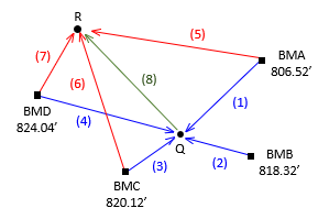 |
| Figure F-5 Level Circuit |
Additional information are the number of instrument setups on each line.
| Obs | Line | dElev | Setups | Obs | Line | dElev | Setups | |
| 1 | BMA-Q | +8.91 | 3 | 5 | BMA-R | -3.56 | 3 | |
| 2 | BMB-Q | -2.92 | 2 | 6 | BMC-R | -17.12 | 4 | |
| 3 | BMC-Q | -4.67 | 1 | 7 | BMD-R | -21.10 | 2 | |
| 4 | BMD-Q | -8.66 | 3 | 8 | Q-R | -12.47 | 3 |
a. Observation equations
The observation equations are the same as in the Chapter D example.

b. Set up matrices
The [C], [U], [K], and [V] matrices are also the same.

Compute weights from number of setups. Weights are inversely proportional to number of setups.
| Obs | Line | Setups | Weight | Obs | Line | Setups | Weight | ||
| 1 | BMA-Q | 3 | 1/3 | 5 | BMA-R | 3 | 1/3 | ||
| 2 | BMB-Q | 2 | 1/2 | 6 | BMC-R | 4 | 1/4 | ||
| 3 | BMC-Q | 1 | 1/1 | 7 | BMD-R | 2 | 1/2 | ||
| 4 | BMD-Q | 3 | 1/3 | 8 | Q-R | 3 | 1/3 |
The weights can be multiplied by 12 to make them integers. The weight matrix is:

c. Solve Unknowns: [U] = [Q] x [CTWK]
Multiply [CT ] x [W] and [CTW] x [C]

Multiply [CTW] x [K]

Invert [CTWC]
Since this is a 2x2 matrix, it can be quickly inverted using its the determinant.

Compute the elevations
Carry enough significant figures to avoid rounding errors.

d. Adjustment Statistics
Residuals: [V] = [CU] - [K]


e. Comparison of Unweighted and Weighted Adjustment
| Point | Unweighted, So=±0.028 | Weighted; So=±0.067 | ||
| Q | 815.418 | ±0.013 | 815.424 | ±0.012 |
| R | 802.962 | ±0.014 | 802.958 | ±0.016 |
Weighing observations changed the elevations changed slightly. Although So increased, it's a better overall indicator of the mixed quality observations.