E. Weights
1. Introduction
The smaller the expected random error in a measurement, the higher its quality. What happens when we combine different quality measurements?
Let's say three crews measured the same distance using different equipment. Their results are:
| Method | Distance | Precision |
| Stadia | 352.11 | 1/400 |
| Steel tape | 351.92 | 1/1000 |
| Total Station Inst (TSI) | 351.35 | 1/10,000 |
What's the distance? We could use a simple average of the three distances:
![]()
Even though, by definition, the MPV is the value which minimizes the sum of the squares of the residuals, is it the best representation of the distance? Although they are of mixed quality, each measurement has the same effect on the MPV. From the precisions, it's obvious the TSI measurement is better that the others, We should allow it greater influence on the MPV. We do this by assigning weights based on measurement quality.
The weighted mean is computed using Equation E-1
 |
Equation E-1 |
|
meas: Measurement |
|
A measurement's weight is related to its error - the smaller the error, the greater the weight. Assuming measurements mistakes and systematic errors have been compensated, precision can be used as an accuracy surrogate. The weight is inversely proportional to the square of its error.Taking the inverse of each precision squared can lead to some pretty big numbers. To keep them reasonably small we can divide each by the lowest weight.
| Method | Distance | Precision | Weight | Weight |
| Stadia | 352.11 | 1/400 | 4002 | 1 |
| Steel tape | 351.92 | 1/1000 | 10002 | 6.25 |
| Total Station Inst (TSI) | 351.35 | 1/10,000 | 10,0002 | 625 |
Based on weights, the MPV is

The MPV is "pulled" toward the TSI measurement since it is the highest quality.
The simple average is sometimes referred to as the unweighted mean. It can also be considered to have unit weighting, that is, the weight of each measurement is 1.
2. Assigning Weights
Weights can have significant impact on an adjustment. When combining multiple measurements in network adjustment, an appropriate weighting strategy should be employed. Weights can be general based on experience or detailed taking onto account multiple error sources for the type of measurement.
If a quantity is measured a sufficient number of times, the standard deviation of the measurement set can be used. How many times must a measurement be repeated for its standard deviation to be statistically significant? It depends.
Specific measurement types have particular random errors affecting their quality. These errors, described in the various Topics and Chapters on measurements, can be used to determine weights.
a. Stategies for Different Measurement Types
(1) Differential Leveling
The elevation difference between points is ( SumBS - SumFS). Weights can be assigned by:
- Number of set ups: Each time a level is set up and readings taken, there is an error potential. If the expected error is similar for each setup, then the more setups between points the greater the potential error (Error of a Series).
- Distance: As sight distances increase, there is greater reading error potential as well as random atmospheric anomolies. Even with balanced sight distances, error also increases on longer point-to-point runs, Figure E-1.
 |
| Figure E-1 Leveling Error Accumulation |
Weights are inversely proportional to number of setups or distance.
(2) Electronic Distance
Primary error sources in electronic distance measurement, Figure E-2, are instrument and reflector centering and the instrument's Manufacturer's Stated Accuracy (MSA).
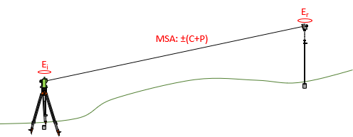 |
| Figure E-2 Electronic Distance Errors |
The MSA is a random error expressed as a "constant" uncertainty along with a proportional uncertainty based on distance. It is expressed as ±(C+P), eg, ±(2 mm + 3 ppm). Equation E-2 are the combined errors,
| Equation E-2 | |
|
Ei: Instrument centering error |
|
A distance weight is inversely proportional to the square of its error.
(3) Horizontal Angles
Angles are among the most complex measurements for which to determine a general weighting strategy. There are multiple random error sources affecting angle quality, Figure E4.
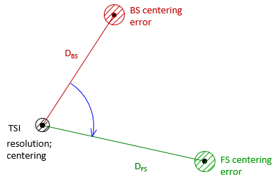 |
| Figure E-4 Angle Error Sources |
These errors are discussed in detail in Chapter D of VII. Total Station Instruments leading up to Equation D-4 of that chapter repeated here as Equation E-3.
| Equation E-3 | |
|
Epr: Pointing and reading error; seconds |
|
Equation E-3 is deceptively subtle as each of the errors under the radical have their own equation taking into account pointings, setups, and instrument specification.
An angle's weight is inversely proportional to the square of its error.
b. Sometimes Science, Sometimes Art
A single weighting strategy for each type of measurement may not be appropriate. Network measurements, particularly horizontal and 3D, can contain a mix of instrumentation, personnel, and conditions. For example, measurements using TSIs with different pointing errors and MSAs should have their own weighting. A differential leveling circuit containing a mix of single- and three-wire observations should not use the same weighting. Even using the same equipment under similar conditions, a seasoned surveyor will probably have better measurements than a novice technician. All this, and more, must be considered for determining weights. Some can be numerically defined, others subjectively based on experience and judgement.
3. The Weight Matrix
Equation E-4 is the general matrix algorithm for observation equations with weight matrix, [W], included; Equation E-5 is the matrix solution for the unknowns.
| Equation E-4 | |
| Equation E-5 |
Because each observation has a weight, [W] is a diagonal m x m matrix, Figure E-5.
 |
| Figure E-5 Weight Matrix |
The iwi element is the weight for the ith observation. Off-diagonal elements are zero.
Since the weight matrix appears on both sides of Equation E-4, it cancels when computing the residuals, Equation E-6.
| Equation E-6 |
Weights are used in the standard deviation of the unit weight computation, Equation E-7.
 |
Equation E-7 |
4. Example
Adjust the same level circuit from Chapter D, Figure F-5.
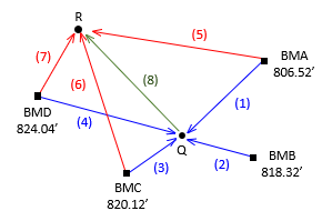 |
| Figure F-5 Level Circuit |
Additional information are the number of instrument setups on each line.
| Obs | Line | dElev | Setups | Obs | Line | dElev | Setups | |
| 1 | BMA-Q | +8.91 | 3 | 5 | BMA-R | -3.56 | 3 | |
| 2 | BMB-Q | -2.92 | 2 | 6 | BMC-R | -17.12 | 4 | |
| 3 | BMC-Q | -4.67 | 1 | 7 | BMD-R | -21.10 | 2 | |
| 4 | BMD-Q | -8.66 | 3 | 8 | Q-R | -12.47 | 3 |
a. Observation equations
The observation equations are the same as in the Chapter D example.

b. Set up matrices
The [C], [U], [K], and [V] matrices are also the same.

Compute weights from number of setups. Weights are inversely proportional to number of setups.
| Obs | Line | Setups | Weight | Obs | Line | Setups | Weight | ||
| 1 | BMA-Q | 3 | 1/3 | 5 | BMA-R | 3 | 1/3 | ||
| 2 | BMB-Q | 2 | 1/2 | 6 | BMC-R | 4 | 1/4 | ||
| 3 | BMC-Q | 1 | 1/1 | 7 | BMD-R | 2 | 1/2 | ||
| 4 | BMD-Q | 3 | 1/3 | 8 | Q-R | 3 | 1/3 |
The weights can be multiplied by 12 to make them integers. The weight matrix is:

c. Solve Unknowns: [U] = [Q] x [CTWK]
Multiply [CT ] x [W] and [CTW] x [C]

Multiply [CTW] x [K]

Invert [CTWC]
Since this is a 2x2 matrix, it can be quickly inverted using its the determinant.

Compute the elevations
Carry enough significant figures to avoid rounding errors.

d. Adjustment Statistics
Residuals: [V] = [CU] - [K]


e. Comparison of Unweighted and Weighted Adjustment
| Point | Unweighted, So=±0.028 | Weighted; So=±0.067 | ||
| Q | 815.418 | ±0.013 | 815.424 | ±0.012 |
| R | 802.962 | ±0.014 | 802.958 | ±0.016 |
Weighing observations changed the elevations changed slightly. Although So increased, it's a better overall indicator of the mixed quality observations.
5. Chapter Summary
A major advantage of LS is the ability to integrate differing quality measurements in an adjustment. Measurements can be apportioned their representative effect on results as long as appropriate weighting is used.
Think of a survey network as a structure, Figure E-6, and weights as stiffness or deformation resistance.
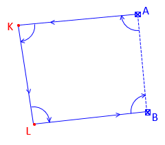 |
| Figure E-6 2D Survey Network |
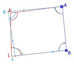
Higher weights add rigidity lowering standard deviations causing points to move less, Figure E-7(a). Lower weights relax the network causing standard deviations to increase allowing points to move more, Figure E-7(b).
 |
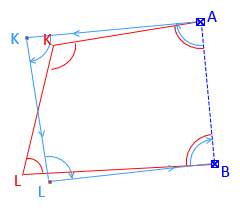 |
| (a) Higher Weights | (b) Lower Weights |
| Figure E-7 Weight Effects |
|
On the other hand, weights that are too high assume minimum measurement errors and allow least point movement. This can provide a false sense of security.
Weights can have a significant impact on adjustment results. While not discussed here, most software provide analysis tools to assist appropriate weight determination. Unit weighting may only be appropriate with direct measurements using the same equipment and personnel under consistent conditions. A network of mixed measurement types and quality should use appropriate weights.
Mixing measurement types, like distances and angles, also mixes dimensions and units; these must cancel correctly or the adjustment results may not make sense. Because distance and angle weights are inversely proportional to errors squared, their squared units are in the denominator of the weight matrix elements. This allows correct unit cancellations in the [CTWC] and [CTK] matrix products.
Accuracy of final positions should reflect the quality of the measurements used to create them.