D. Matrix Method
1. General
The Matrix method is a third way to perform an LS adjustment, using matrix algebra incorporating principles in the XIV. Simultaneous Equations topic.
The baisc premise for all three methods is the same: minimizing the sum of the squares of the residuals. The methods differ in how that is achieved. The Brute Force method begins with averages since those statistically meet the minimization criterion. The Direct Minimization method starts with observation equations written in terms of residuals, which are then minimized by derivation, and unknowns solved simultaneously.
The Matrix method is an extension of Direct Minimization using observation equations to build matrices, manipulate them, and solve simultaneous equations.
2. Equation Solution using Matrices
Observation equations can be written in the form [C] x [U] = [K]. Using n for the number of unknowns and m for the number of observations, the matirces dimensions are:
| n[U]1 | m[K]1 | m[V]1 |
The unknowns in the U matrix are solved using the matrix algorithm Equation D-1:
| [U] = [CTC]-1 x [CTK] | |
|
[Q] = [CTC]-1 |
|
| [U] = [Q] x [CTK] | Equation D-1 |
[Q] is a symmetric m x m matrix; [CTK] is a m x 1 matrix. Equation D-1 is a simultaneous solution of m equations in m unknowns.
Because there are redundant measurements, a residual term is added to each observation equation so the matrix algorithm is [C] x [U] = [K] + [V]. Residuals are computed after the adjustment using Equation D-2.
| [V] = [CU] -[K] | Equation D-2 |
3. More Statistics
a. Propagating Error
We saw that Brute Force doesn't work when unknowns are directly connected with measurements. In the Direct Minimization method, connected unknowns appear in the same partial derivatives. Although the standard deviation of unit weight, So, for overall adjustment can be computed in both methods, neither allows easy determination of the expected quality of their individually adjusted values.
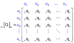
The Matrix method allows So to be propagated into the adjusted values with the covariance matrix, [Q] . It is used to compute expected standard errors of adjusted unknowns or adjusted observations. The corresponding unknowns for the [Q] matrix in Figure D-1 are u1, u2, u3, ... un.
 |
| Figure D-1 Covariance Matrix |
b. Standard Errors of Adjusted Values
Each covariance matrix diagonal element is unique to one of the unknown quantities and is used to compute its expected error, Equation D-3.
| Equation D-3 |
c. Standard Errors of Adjusted Observations
An adjusted observation is computed by adding its residual to the original observation, Equation D-4.
| Equation D-4 | |
|
i: observation number |
|
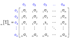
Uncertainties of the adjusted observations are related by the observation coefficients, covariance matrix, and So. The cofactor matrix, [Σ], is a product of the [C], [Q], and [CT] matrices, Equation D-5.
| Equation D-5 |
The size of the cofactor matrix is m x m, Figure D-2, so it can be quite large if there are many observations.
 |
| Figure D-2 Cofactor Matrix |
The standard error of an observation is computed with Equation D-5.
| Equation D-5 | |
|
iσi : Diagonal element of [Σ] for observation i |
|
Because only a diagonal element is needed, the computations can be reduced somewhat. Each row of the [C] matrix corresponds to a particular observation. Because [CT] is the transpose of [C], each of its columns correspond to the same observations, Figure D-3.
 |
| Figure D-3 [C] and [CT] Matrices |
An observation's [Σ] matrix diagonal element can be computed using its [C] row and [CT] column with the [Q] matrix, Equation D-6.
| Equation D-6 | |
|
i: observation number |
|
Equation D-7 is Equations D-5 and D-6 combined.
| Equation D-7 |
4. Example
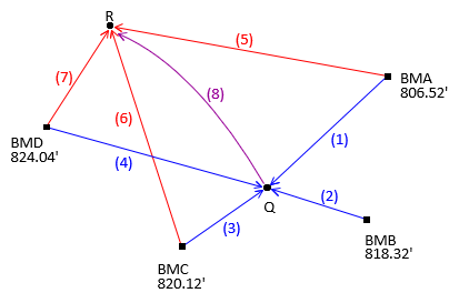
Adjust the level circuit of Chapter C shown in Figure D-2.
 |
| Figure D-2 Level Circuit |
| Obs | Line | dElev | Obs | Line | dElev | |
| 1 | BMA-Q | +8.91 | 5 | BMA-R | -3.56 | |
| 2 | BMB-Q | -2.92 | 6 | BMC-R | -17.12 | |
| 3 | BMC-Q | -4.67 | 7 | BMD-R | -21.10 | |
| 4 | BMD-Q | -8.66 | 8 | Q-R | -12.47 |
(1) Observation Equations
Use Equation D-4 as the initial observation equation format, then rearrage to place the unknowns on the left side, constants and residuals on the right.
| Equation D-43 |

(2) Set up Matrices

(3) Solve Unknowns: [U] = [Q] x [CTK]
[CT] x [C]

[CT] x [K]

Invert [CTC] to get [Q]

[Q] x [CTK]

These are the same elevations as in the Direct Minimization method.
(4) Adjustment Statistics
Residuals: [V] = [CU] - [K]

Compute So

![]()
Standard deviations for points Q and R elevations using Equation D-2

Adjusted observations

Adjusted observation uncertainties using Equation D-7.
Obs 1
First row of [C] and first column of [CT].

Because rows 1-4 of the C matrix are the same, all four observations will have the same expected error.
Ditto for observations 5-7
Obs 5
Fifth row of [C] and fifth column of [CT].

Obs 8
Eighth row of [C] and eighth column of [CT].

Outside of having the same [C] coefficients, why do observations 1-5 have the same expected errors? Because each connects a benchmark to the adjusted point Q (that's why they have same rows in [C]). The only error affecting those observations is point Q's. Similarly, observations 5-7 are only affected by point R. Only the eighth observation has uncertainties at both ends.
(5) Adjustment Summary
Degrees of freedom: DF = 8-2 = 6
Std Dev Unit Wt: So = ±0.028
Adjusted elevations
| Point | Elevation | Std Dev | |
| Q | 815.418 | ±0.013 | |
| R | 802.962 | ±0.014 |
Adjusted observations
| Line | Adj Obs | SE |
| BMA-Q | 8.898 | ±0.013 |
| BMB-Q | -2.902 | ±0.013 |
| BMC-Q | -4.702 | ±0.013 |
| BMD-Q | -8.622 | ±0.013 |
| BMA-R | -3.558 | ±0.014 |
| BMC-R | -17.158 | ±0.014 |
| BMD-R | -21.078 | ±0.014 |
| Q-R | -12.456 | ±0.017 |
5. Chapter Summary
Advantages of the Matrix method include
- Systematic adjustment process
- Error propagation for adjusted values and observations
Like the Direct Minimization method, measurements between unknowns are easily included. However, instead of taking derivatives, observation equation values are added as rows to the [C] and [K] matrices. This alone can make a big difference with non-linear observation equations which can have up to six partial derivatives each.