E. Level Network Adjustment
1. Misclosure
a. Determining
A closed level network is either a loop or link which begins and ends on a known elevation, Figure E-1.
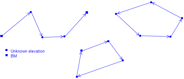 |
| Figure E-1 |
In the process of running the network, new elevations are measured including that of the known ending elevation. The difference between the known and measured ending elevation allows us to determine the amount of error, or misclosure, in the network:
| M =(Known End Elev) - (Meas'd End Elev) | Equation E-1 |
| M: misclosure | |
Misclosure should be the result of accumulated random errors. Systematic errors and mistakes must be eliminated first in order to judge quality of the newly created elevations. Random errors, while they can't be entirely eliminated, can be minimized by knowledgeable personnel using the appropriate equipment and procedures under the best conditions.
b. Allowable
How much misclosure is acceptable? It depends on the purpose of the network. The allowable misclosure should be consistent with how random errors accumulate. Differential leveling consist of a series of instrument setups at which two rod readings are made. This is repeated throughout the entire network. If we assume that each time the process is performed we expect a certain error behavior then we can consider the total misclosure to behave like an Error of a Series.
 |
Equation E-2 |
|
c: total error |
|
(1) Formal standards
Table E-1 is taken from Section 3.5 Geodetic Leveling of Standards and Specifications for Geodetic Control Networks, FGCC, 1984.
| Table E-1 |
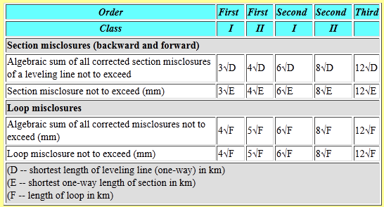 |
The Loop misclosure not to exceed (mm) row identifies the network misclosure using a form of the Error of a Series equation. The allowable misclosure is based on the loop length (that is, the total of all the BS and FS distances) instead of instrument set ups. Consider the greater difficult reading a level rod at twice the distance - not only are rod divisions smaller but other environmental factors add to the difficulty as well. Assuming error accumulates as a function of distance is reasonable.
Example
The distance around a level network is approximately 1800 ft. What is the allowable misclosure, in feet, if the network is to meet Second Order Class II standards?
Convert the distance to km

Compute the misclosure, m, and convert to feet

(2) Informal standards
Informal standards can also be based on the Error of a Series. However, the error accumulation could be presumed based on distance surveyed or number of instrument setups.
Example
A survey crew ran a level network consisting of seven set ups. If they have an expected error of ±0.005 ft for each set up, what is their expected network misclosure?
Using Equation E-2:

Whether using formal or informal standards, remember that the final results are affected by errors from the different sources. Controlling those errors is paramount to meeting misclosure standards by design, not by mistake.
2. Network Adjustment Methods
Network adjustment is the method by which the misclosure is distributed back into the newly created elevations. The adjustment methodology should reflect error behavior and be repeatable. There are a number of approaches, some better than others. These are summarized in Table E-2.
| Table E-2 | |||
| Method | Premise | Advantage | Disadvantage |
| Ignore | Don't adjust anything. | Simple; repeatable. | Ignores errors. |
| Arbitrary | Place error randomly in one or more raw elevations. | Simple. | Not repeatable. |
| Judgement call | Decide based on field conditions, equipment, and personnel, which raw elevations probably had more error. | Considers error behavior. | Not repeatable; not rigorous; requires personal knowledge of entire project. |
| Equal distribution | Distribute errors equally among raw elevations. | Simple; repeatable. | Treats random errors systematically; assumes all errors are positive or negative. |
| Proportional distribution | Distribute errors based on sight distances. | Simple; repeatable; accounts for greater error in longer sights. | Treats random errors systematically; assumes all errors are positive or negative; requires distances. |
| Least squares | Full statistical approach. | Allows full random error modeling; can mix different quality measurements; provides adjusted elevation uncertainties. | Most complicated and computation-intensive. |
For simple networks, Figure E-2(a), the Equal or Proportional distributions generally give satisfactory results. However in complex networks which have additional measurements between points, Figure E-2(b), using the Equal or Proportional methods is too cumbersome if not impossible.
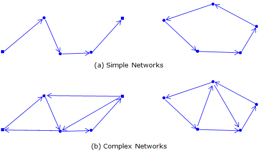 |
| Figure E-2 |
In a simple network, each point has only a single raw elevation. In a complex network, each point can have multiple raw elevations based on connections to other points. The raw elevations differ because their respective random errors accumulated along different paths to the point. The best way to model and compensate the errors is using least squares.
The concept of least squares is beyond the scope of this discussion since we are limiting it to simple networks. We will look at applying the Equal and Proportional methods.
3. Network adjustment example 1
a. Data
A level network, Figure E-3, starts at BM Q, whose elevation is 820.12 ft, travels to points A, TP1, B, and closes back on BM Q. The raw field elevations are shown on the diagram; red numbers are the total of the BS and FS distances between points.
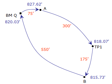 |
| Figure E-3 |
From Equation E-1, the network misclosure is: M = 820.03 ft - 820.12 ft = -0.09 ft
b. Equal distribution
The Equal distribution applies an equal part of the misclosure to each raw elevation. It is a cumulative correction since each corrected elevation affects following raw elevations by a like amount.
 |
Equation E-3 |
| M: misclosure n: number of raw elevations determined i: elevation number |
|
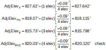
Four raw elevations were established counting the closing elevation on BM Q. Substituting this network's values in Equation E-1:

“i” is the sequential number of each elevation in the order they were created; A is 1, TP1 is 2, etc.
The adjusted elevations (computed to an additional decimal place minimizing rounding error) are:
c. Proportional distribution
The Proportional distribution applies a part of the misclosure to each raw elevation based on sight distances. It is also a cumulative correction since each corrected elevation affects following raw elevations by a like amount.
 |
Equation E-4 |
| M: misclosure D: total BS and FS distances d: cumulative distance to current point |
|
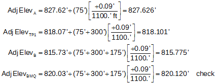
The total distance, D, around the loop is 75'+300'+175'+550' = 1100'. Setting up Equation E-2 for this network:

The adjusted elevations (computed to an additional decimal place minimizing rounding error) are:
d. Comparison
Table E-3 is a summary comparison of the point elevations from the two methodes.
| Table E-3 | ||
| Point | Equal | Proportional |
| A | 827.642 | 827.626 |
| TP1 | 818.115 | 818.101 |
| B | 815.798 | 815.775 |
| BM Q | 820.120 | 820.120 |
e. Comments
(1) Math check
Computing back into BM Q for both methods provides a math check. A common mistake is to forget to reverse the sign of the misclosure. If that were the case, the adjusted elevation at BM Q would be 0.18' too low - twice what it was indicating corrections were applied in the wrong direction.
(2) Skipping points
Although the adjusted elevation of TP1 was computed in both methods, it can be skipped since it's only a temporary point. However, any elevation determined in the field, temporary or permanent, must be included in the count (n) for the Equal distribution and the distances through them for the Proportional distribution.
(3) Same results?
If the sight distances between points are all equal then the Proportional distribution will result in the same adjusted elevations as the Equal distribution.
(4) Random errors only
Misclosure is a result of random errors - mistakes must removed and systematic errors compensated. If they aren’t, then the quality of the adjusted elevations will be degraded. For example, assume the same network but the closing elevation for BM Q was 825.10', 4.98' too high, Figure E-3. A misclosure that large is usually the result of one or more mistakes.
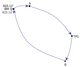 |
| Figure E-4 Network with a Mistake |
Using an Equal distribution, the equation set up is:

If the error occurred between TP1 and B, the raw elevations of A and TP1 won’t be affected by it. Nor will the raw elevation difference between B and BM Q.
If the network is adjusted without first eliminating the mistake, then parts of it will be pushed into all raw elevations. Instead of isolating the error, its effect is spread through the entire network.
If the misclosure is larger than reasonable, look for mistakes or unresolved systematic errors. If neither can be found, or the misclosure is still unreasonably large, then part or all of the network may need to be re-run.
4. Network adjustment example 2
a. Data
The diagram below shows a link circuit running from BM Lima to BM Hotel.
are instrument locations.
TP# is a temporary turning point.
Green numbers are elevations determined in the field.
Blue numbers are BS and FS distances in paces measured by the rod person.
The rod person's pace count is 41.5 paces per 100.0 ft.
Known elevations are BM Lima = 926.49' and BM Hotel = 953.41'
Because the network ended on BM Hotel, we use its measured and known elevations to determine the misclosure, M:
M=953.49' - 953.41'= +0.08'
b. Equal distribution
A total of 7 elevations were established. From Equation E-1:

Applying the equation to each non-turning point:


We don't need to adjust the turning point elevations, we just need to keep track of the sequential number of the elevation that is being adjusted. As a math check, we always compute the adjusted elevation of the closing point.
c. Proportional distribution
The total sight length of the network is:
(53p+54p+39p+39p+62p+61p+46p+47p+29p+28p+66p+68p+31p+32p) = 655p
We could use the rod person's pace count to convert 655p to feet, but we don't need to. Why not? Because the paces will cancel in the elevation adjustment equation.
From Equation E-2:

To adjust the elevation of A:

Cumulative and total distance units cancel.
Before continuing with the rest, let's compute the cumulative distance to each point so our adjustment equations don't become too cumbersome.
A: 54p+54p = 107p
TP1: 107p+39p+39p = 185p
B: 185p+62p+61p = 308p
TP2: 308p+46p+47p = 401p
C: 401p+29p+28p = 458p
D: 458p+66p+68p = 592p
BM Hotel: 592p+31p+32p = 655p


Although we didn't adjust turning points elevations, we included the distances through them to points that were adjusted.
