3. Network Adjustment

a. Simple Adjustments for Simple Networks

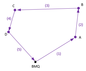
Random errors must be distributed back into the measurements, preferably in a manner mirroring their accumulation. For many basic survey projects with just enough measurements to determine misclosure, manual adjustment methods using a simplified approach are generally applied. The level circuit in Figure A-13(a) can be easily adjusted by applying equal or distance-based proportional corrections. Likewise the lot traverse misclosure in Figure A-13(b) can be adjusted by distributing the errors proportionately into each line's latitude and departure which in turn changes each measured angle and distance.

(a) Simple Loop Circuit	(b) Simple Lot Traverse
Figure A-13 Survey Networks

In either case, the closure errors, which are random, are treated systematically. Simple adjustments treat each error correction the same: all are added or subtracted. Random errors can be positive or negative so some corrections should be added, others subtracted. Simple networks do not have sufficient information to distribute the errors in like fashion.

b. Adding Redundancy

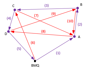
Increasing the number of measurements, ie, redundancy, provides random errors greater opportunity to cancel, theoretically lowering misclosure errors. A disadvantage is that simple adjustment methods to distribute random errors are difficult, if not impossible, to apply. Figure A-14 show the previous level and traverse networks with additional measurements.

(a) Level Circuit	(b) Traverse
Figure A-14 Measurements Added

Consider the measurements as "paths" along which misclosure can be computed. For example, in Figure A-12(a), level misclosure can be computed following the original path, BMQ-A-B-C-D-A-BMQ, or BMQ-A-B-C-A-D-BMQ, or BMQ-C-A-B-D-BMQ, or ..., etc.  Because of random error behavior, each path will probably have a different misclosure. Using a simple adjustment along each path will likely result in each point having multiple adjusted elevations. For example, how many paths can be defined which connect point C to the benchmark? They needn't go through other points, just begin and end on the benchmark. If we adjust the elevation of point C using every path through it, theoretically their average would be the "best" elevation.
Of course, that can be a lot of computations.
The same logic can be applied to the traverse in Figure A-12(b) with similar results.

Additional measurements don’t faze a Least Squares (LS) adjustment; as a matter of fact, the more the merrier. More measurements strengthen a network, provide more random error compensation opportunity, and lead to better adjusted values. Major LS adjustment benefits are:

• Adjusted values based on appropriate random error behavior
• Quality estimates of adjusted values
• Better integration of and accounting for different quality measurements

There are, however, downsides to LS:

• It can be extremely computation-intensive, usually requiring specialized software.
• It is easy for the user to become lost trying to interpret adjustment results.
• Like any computational tool, least squares can be misapplied.

c. Random Errors Only

Network misclosures should be the result of random errors. Specific field procedures are followed, measurement conditions compensated, and measurements repeated to eliminate mistakes and compensate systematic errors. Standards and specifications are used to ensure remaining errors are within an acceptable limit.

If an undiscovered mistake is included in an adjustment, its effect can be spread throughout the network beyond just the measurement where it occurred. This is true not just for a simple adjustment, but also an LSA. Unlike a simple adjustment, an LS adjustment provides statistics which can help identify if a mistake has been included and possibly where it occurred. Unresolved systematic errors, however, may be more difficult to find. For example, if incorrect atmospheric conditions were used for a total station survey, all distances would be proportionately affected the same, like a scale factor. Neither a simple adjustment nor LS would detect the non-random error.

Whether simple or complex, an adjustment must be applied only to random errors.

d. Least Squares

(1) Basic Premise

When there are multiple values for the same quantity, a decision must be made which singular representative value will be used. Topic II. Errors  Chapter F. Random Errors discussed basic statistics and indicated the arithmetic average as the most probable value (MPV) of a measurement set. It didn't explain why the MPV is used and the derivative mathematics behind it are beyond the scope of this basic LS discussion.

Recall that a residual is the difference between the MPV and an individual measurement, Equation A-4. Because the MPV is the average, the sum of the residuals tend to zero. The larger the measurement set, the closer to zero. The basic premise of LS is that the sum of the squares of the residuals is minimized, Equation A-5. It is the least sum of the sum of residuals squared - least squares, get it?

		Equation A-4
		Equation A-5
	MPV: Most Probable Value o: Observation v: Residual m: Number of measurements

The purpose of network adjustment is to use all measurements to simultaneously determined the MPV for all unknowns.

(2) Quality Indicators

Standard deviation is a quality indicator of precision. If mistakes have been eliminated and systematic errors compensated, the residuals closely approximate errors. Because of this, most data adjustment texts tend to use the terms standard deviation and standard error interchangeably. 

(a)  Adjustment

For direct measurements standard deviation, S, is determined using Equation F-2 in Topic II. Errors  Chapter F, repeated here as Equation A-6.

		Equation A-5
	v: Residual m: Number of values

The situation differs for indirect measurements with multiple unknowns in a network. The Standard Deviation of the Unit Weight, S_o, Equation A-6, is an indicator of overall network adjustment quality

		Equation A-6
	v: Residual m: Number of observations n: Number of unknowns

(b) Adjusted Quantities

Adjusted quantities in a network include the unknowns and the observations connecting them.

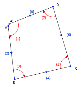
For example, the unknowns in the level circuit of Figure A-15 are the elevations of points R and A, the observations are dE₁, dE₂, and dE₃.

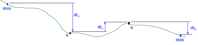Figure A-15 Unknowns and Observations

After adjustment, each elevation will have an estimated accuracy. Differences between adjusted elevations are the adjusted observations. The elevation uncertainties are propagated into the adjusted observations, Figure A-16.

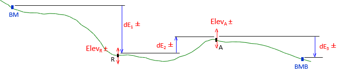Figure A-16 Adjusted Observations

As with direct measurements, the more redundancies in a network, the stronger its overall geometry.