A. Introduction

1. Direct and Indirect Measurements

We discussed direct and indirect measurements waaaay back in I. Basic Principles. We'll briefly review their concepts here because most of what the surveyor does, in total, consists of indirect measurements.

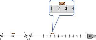
Using a measuring device on an unknown quantity to determine its value is direct measurement. The value is determined comparing the device to the quantity and reading the value from gradations or a digital display. Examples include measuring:

• a distance with a tape, Figure A-1
• an angle with a total station
• atmospheric pressure using a barometer.

Outside of applying systematic error corrections, no computations are necessary to determine the value from the measurement.

Figure A-1 Distance Taping

Indirect measurements are used with computations to determine an unknown quantity. Examples include:

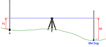
• elevation determination using backsight and foresight readings, Figure A-2
• spot elevations by three dimensional surveying
• lot area from angles and distances

These are typically networks: one or more types of measurements combined with computations to determine desired value(s). We will use the term in this context when discussing network adjustment in the rest of this topic.

Figure A-2 Differential Leveling

Direct and indirect measurements affect how errors propagate into the quantity being determined.

2. Redundancy

a. Something Extra

When something is redundant, it is generally thought unnecessary. In a way, it is, but in measurement science, a redundancy is something extra that we try to give effect to. We routinely include extra measurements in surveying, for a few different reasons. Two are illustrated here with direct and indirect measurement examples.

b. Direct Measurement: Taping

Consider measuring a lot line once with a 100 ft steel tape. With the tape supported along its entire length and a carefully applied consistent 20 pound pull, the result is 362.24 ft. Can the length be reliably stated as 362.24 ft?

The distance is measured a second time, on a day colder by 25°F, with same support and pull, but this time the result is 262.19 ft. What happened? Did the distance actually shrink because of the temperature change?

If you have ever used a steel tape, you will immediately realize part of the problem: the number of full tape lengths was apparently miscounted. Either an extra full tape length was included in the first measurement or omitted from the second. Either way, a mistake was made. So how to resolve it? By measuring a third time and hoping it matches one of the first two.

If the third measurement is 362.36 ft, that means the second measurement has (at least) a full tape length mistake. We can either discard the second measurement or "correct" it by adding 100 ft. If we discard it, there's still a 0.12 ft difference between the first and last measurements. Much of this can be attributed to the temperature change which is a systematic error: the tape shrank at a lower temperature making the measurement too long. Once this and other systematic errors are compensated, the only errors left are random.

A single measurement of an unknown quantity is a unique solution - there is only one possible value for the unknown. Any measurement beyond the first is redundant. In this taping example, a second redundant measurement revealed a mistake existed, a third helped isolate it..

Should we automatically discard any measurements that contain a mistake? It could depend on the situation. In this example, assuming a tape mis-count happened, adding a full tape length makes the second measurement 362.19 ft which is consistent with the other two. Had it been 275.69 ft, an omitted 100 ft tape length doesn't account for the difference; something else happened. In either case, multiple measurements help identify where the mistake occurred. The safest thing to do is discard the mistaken measurement.

c. Indirect Measurement: Leveling

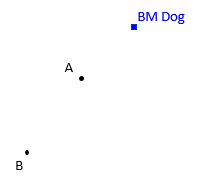
Let's look at the example of a simple differential level circuit. Elevations of points A and B are to be determined from a benchmark, BM Dog, Figure A-3.

Figure A-3 Leveling Circuit

Differential leveling consists of a sequence of backsight (BS) and foresight (FS) rod readings, Figure A-4.

Figure A-4 Differential Leveling

BS readings are added, FS subtracted to get the total elevation difference along a line, Equation A-4.

Equation A-1 Equation A-2

In general terms, an observation is a measurement with which an unknown quantity can be determined. In this case specifically, it is the elevation difference dElev_DA from BM Dog to point A, Equation A-2. Because the intermediate points are temporary, dElev_DA is the sum of the FS readings subtracted from the sum of the BS readings, Equation A-1.

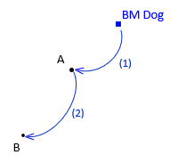
How many observations are necessary to determine the elevations of points A and B? Technically only two: one from BM Dog to A, another from A to B, Figure A-5.

Figure A-5 Connecting A to BM Dog

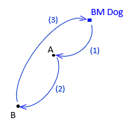
There are two unknown elevations and two measurements making this a unique solution. As with the taping example, the primary issue with a unique solution is insufficient information to determine if errors are present nor what kind they are. For example, a rod reading error would be undetectable. To address this, surveyors typically close a level circuit back to the original benchmark or another benchmark in the same vertical system, Figure A-6

Figure A-6 Closing the Circuit

This third observation back to the benchmark is a redundancy allowing misclosure determination. A redundancy is also called a Degree of Freedom (DF). The number of DF are determined from Equation A-3.

		Equation A-3
	DF: Number of degrees of freedom m: Number of observations n: Number of unknowns

DF must be equal to or greater than 0 or the unknowns cannot be solved. DF = 0 is a unique solution with no redundancy.
The sum of the three observations in Figure A-6 is the misclosure, its size depending on errors.

• A large difference indicates the presence of one or more mistakes.
• A smaller difference, but one outside some acceptable misclosure limit, could be the result of uncompensated systematic errors. For example, using a level with a collimation error and not balancing BS and FS distances.
• A small difference within an allowable misclosure limit is caused by random errors.

d. True or Pseudo Redundancies

Having redundancies alone is not sufficient, they must be the right kind. We can distinguish between true and pseudo redundancies.
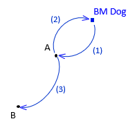
To the circuit of Figure A-3, a third observation is added from A back to the benchmark., Figure A-7.

Figure A-7 Pseudo Redundancy

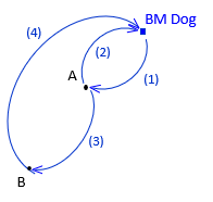
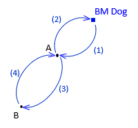
There are two unknowns and three observations resulting in 3-2 = 1 DF. But point B is connected to point A with only one observation. Errors in that observation cannot be trapped. Even though we have one degree of freedom, it's for the section between BM Dog and point A so it isn't a true redundancy for the entire circuit. Another observation must be added connecting point B to the benchmark or to point A, Figure A-8.

(a) DF = 4-2 = 2	(b) DF = 4-2 = 2
Figure A-8 Redundancies Options

Each point must be connected to the network by at least two observations for true redundancy. More observations, more DF, Figure A-9.

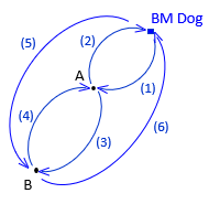Figure A-9 DF = 6-2 = 4

e. Independent Observations

Observations should be made independently of each other as much as possible to avoid repeating the same errors. Simply glancing away and then re-reading the instrument without changing anything does not constitute an independent measurement. A simple level loop between BM and point R, Figure A-10, has one redundancy.

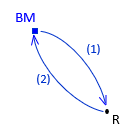Figure A-10 Simple Loop

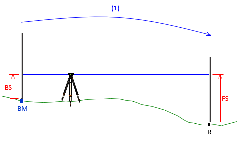
In this case, the  surveyor had an unbalanced sight distance set up for the first observation, Figure A-9(a). After taking BS and FS readings, he left the instrument in place and simply reversed his readings, Figure A-11(b).

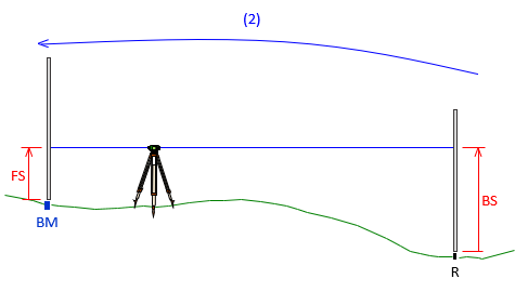Figure A-11 Simple Loop Observations

These are not independent observations. If the instrument had a collimation error, Figure A-12, there is an unresolved systematic error.

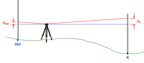Figure A-12 Collimation Error

The circuit would have a near perfect misclosure because both errors are added and subtracted so they cancel:

The only thing affecting misclosure are rod reading errors which are random.
Even though the misclosure may be acceptable, the elevation of point R is incorrect due to the collimation error:

Without independent observations (and correct field procedures) mistakes and systematic errors may not be found.

3. Network Adjustment

a. Simple Adjustments for Simple Networks

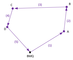
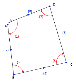
Random errors must be distributed back into the measurements, preferably in a manner mirroring their accumulation. For many basic survey projects with just enough measurements to determine misclosure, manual adjustment methods using a simplified approach are generally applied. The level circuit in Figure A-13(a) can be easily adjusted by applying equal or distance-based proportional corrections. Likewise the lot traverse misclosure in Figure A-13(b) can be adjusted by distributing the errors proportionately into each line's latitude and departure which in turn changes each measured angle and distance.

(a) Simple Loop Circuit	(b) Simple Lot Traverse
Figure A-13 Survey Networks

In either case, the closure errors, which are random, are treated systematically. Simple adjustments treat each error correction the same: all are added or subtracted. Random errors can be positive or negative so some corrections should be added, others subtracted. Simple networks do not have sufficient information to distribute the errors in like fashion.

b. Adding Redundancy

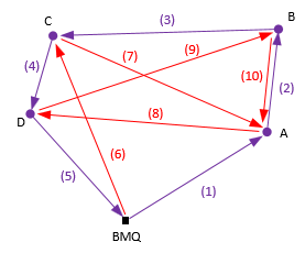
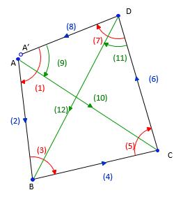
Increasing the number of measurements, ie, redundancy, provides random errors greater opportunity to cancel, theoretically lowering misclosure errors. A disadvantage is that simple adjustment methods to distribute random errors are difficult, if not impossible, to apply. Figure A-14 show the previous level and traverse networks with additional measurements.

(a) Level Circuit	(b) Traverse
Figure A-14 Measurements Added

Consider the measurements as "paths" along which misclosure can be computed. For example, in Figure A-12(a), level misclosure can be computed following the original path, BMQ-A-B-C-D-A-BMQ, or BMQ-A-B-C-A-D-BMQ, or BMQ-C-A-B-D-BMQ, or ..., etc.  Because of random error behavior, each path will probably have a different misclosure. Using a simple adjustment along each path will likely result in each point having multiple adjusted elevations. For example, how many paths can be defined which connect point C to the benchmark? They needn't go through other points, just begin and end on the benchmark. If we adjust the elevation of point C using every path through it, theoretically their average would be the "best" elevation.
Of course, that can be a lot of computations.
The same logic can be applied to the traverse in Figure A-12(b) with similar results.

Additional measurements don’t faze a Least Squares (LS) adjustment; as a matter of fact, the more the merrier. More measurements strengthen a network, provide more random error compensation opportunity, and lead to better adjusted values. Major LS adjustment benefits are:

• Adjusted values based on appropriate random error behavior
• Quality estimates of adjusted values
• Better integration of and accounting for different quality measurements

There are, however, downsides to LS:

• It can be extremely computation-intensive, usually requiring specialized software.
• It is easy for the user to become lost trying to interpret adjustment results.
• Like any computational tool, least squares can be misapplied.

c. Random Errors Only

Network misclosures should be the result of random errors. Specific field procedures are followed, measurement conditions compensated, and measurements repeated to eliminate mistakes and compensate systematic errors. Standards and specifications are used to ensure remaining errors are within an acceptable limit.

If an undiscovered mistake is included in an adjustment, its effect can be spread throughout the network beyond just the measurement where it occurred. This is true not just for a simple adjustment, but also an LSA. Unlike a simple adjustment, an LS adjustment provides statistics which can help identify if a mistake has been included and possibly where it occurred. Unresolved systematic errors, however, may be more difficult to find. For example, if incorrect atmospheric conditions were used for a total station survey, all distances would be proportionately affected the same, like a scale factor. Neither a simple adjustment nor LS would detect the non-random error.

Whether simple or complex, an adjustment must be applied only to random errors.

d. Least Squares

(1) Basic Premise

When there are multiple values for the same quantity, a decision must be made which singular representative value will be used. Topic II. Errors  Chapter F. Random Errors discussed basic statistics and indicated the arithmetic average as the most probable value (MPV) of a measurement set. It didn't explain why the MPV is used and the derivative mathematics behind it are beyond the scope of this basic LS discussion.

Recall that a residual is the difference between the MPV and an individual measurement, Equation A-4. Because the MPV is the average, the sum of the residuals tend to zero. The larger the measurement set, the closer to zero. The basic premise of LS is that the sum of the squares of the residuals is minimized, Equation A-5. It is the least sum of the sum of residuals squared - least squares, get it?

		Equation A-4
		Equation A-5
	MPV: Most Probable Value o: Observation v: Residual m: Number of measurements

The purpose of network adjustment is to use all measurements to simultaneously determined the MPV for all unknowns.

(2) Quality Indicators

Standard deviation is a quality indicator of precision. If mistakes have been eliminated and systematic errors compensated, the residuals closely approximate errors. Because of this, most data adjustment texts tend to use the terms standard deviation and standard error interchangeably. 

(a)  Adjustment

For direct measurements standard deviation, S, is determined using Equation F-2 in Topic II. Errors  Chapter F, repeated here as Equation A-6.

		Equation A-5
	v: Residual m: Number of values

The situation differs for indirect measurements with multiple unknowns in a network. The Standard Deviation of the Unit Weight, S_o, Equation A-6, is an indicator of overall network adjustment quality

		Equation A-6
	v: Residual m: Number of observations n: Number of unknowns

(b) Adjusted Quantities

Adjusted quantities in a network include the unknowns and the observations connecting them.

For example, the unknowns in the level circuit of Figure A-15 are the elevations of points R and A, the observations are dE₁, dE₂, and dE₃.

Figure A-15 Unknowns and Observations

After adjustment, each elevation will have an estimated accuracy. Differences between adjusted elevations are the adjusted observations. The elevation uncertainties are propagated into the adjusted observations, Figure A-16.

Figure A-16 Adjusted Observations

As with direct measurements, the more redundancies in a network, the stronger its overall geometry.