F. Electronic Distance Measurement
1. Electromagnetic Energy
The electromagnetic principles of Electronic Distance Measurement (EDM) theory and operation are well covered in most Surveying text books and on the internet. The intent here is to give the reader a general understanding of EDM so that error sources are better understood and controlled.
An EDM uses electromagnetic (EM) energy to determine the length of a line. The energy originates at an instrument at one end of a line and is transmitted to a reflector at the other end from where it is returned to the originating instrument. The nature of the reflector is dependent on the type of EM.
If electro-optical (infrared or laser) EM is used, Figure F-1, then the "reflector" is typically a passive device which bounces the signal back to the transmitter.
If the EM is microwave, Figure F-2, then the reflector is a second instrument which captures the incoming energy and re-transits it back to the originating instrument.
 |
|
Figure F-1 |
 |
| Figure F-2 Microwave EDM |
In either case the measurement is the total distance from the instrument to the reflector and back to the instrument.
We will limit discussion to electro-optical EM instruments since the majority of EDMs and Total Stations employ that EM type.
2. Distance Determination
An EDM uses the EM signal structure and determines distance using a phase shift. The EM signal has a sinusoidal wave form. Remember from trigonometry that the sine curve looks like, Figure F-3:
 |
| Figure F-3 Sine Curve |
This wave form repeats every 360°. The distance between wave form ends is the wavelength, λ, Figure F-4.
 |
| Figure F-4 Wavelength |
Different wavelengths are generated at different modulation frequencies, f. Wavelength, frequency, and the speed of light are related by:
| λ = c/f | Equation F-1 | |
| λ: wavelength c: speed of light f: frequency |
||
The wavelength is a known quantity since it is generated by the EDM at a specific frequency. The signal leaves the EDM at 0° phase, goes thru N number of full phases on its path to then from the reflector, and returns to the EDM at some angle between 0° and 360° creating a partial wavelength, p, Figure F-5:
 |
| Figure F-5 Phase Shift |
The EDM can very accurately determine the length of the last partial wavelength from its phase. The total EDM-reflector-EDM distance is (Nλ + p).
Example: The wavelength in Figure F-5 is 20.00 ft.There are 10 full wavelengths before the last partial one. What is the EDM to reflector distance?
The last partial wave is: p = (82°30'39.9"/360°00'00") x 20.00 ft = 4.584 ft
Including the full wavelengths the total distance EDM-reflector-EDM is: 10 x 20.00 ft + 4.854 ft = 204.584 ft
The distance between the EDM and reflector is half that: 204.584 ft / 2 = 102.292 ft.
Unfortunately, while the EDM can accurately measure the last partial wavelength, it doesn't know how many full wavelengths occurred before it (this is similar to the integer ambiguity in carrier-based GPS measurements).
So how does the EDM resolve this dilemma?
By decreasing the frequency by a factor of 10 and repeating the process. Decreasing the frequency by a factor of 10 increases the wavelength by a like amount. The partial wavelength at this level will give the next higher distance digit. This is repeated a number of times until the distance is resolved.
Figure F-6 illustrates three frequencies each folded out to show a continuous EDM-reflector-EDM path:
 |
| Figure F-6 Multiple Frequencies |
Example: The following table shows the last partial length for each of 4 different wavelengths. What is the total distance EDM-reflector?
| λ, m | p, m | dist, m |
| 10.00 | 3.68 | |
| 100.0 | 53.7 | |
| 1,000 | 454 | |
| 10,000 | 8450 |
The digits in bold represent the digits added to the distance as a result of each partial wavelength.
| λ, m | p, m | dist, m |
| 10.00 | 3.68 | 3.68 |
| 100.0 | 53.7 | 53.68 |
| 1,000 | 454 | 453.68 |
| 10,000 | 8450 | 8453.68 |
The total distance is 8456.68 m; the EDM-reflector distance is 8453.68/2 = 4226.84 m
3. Distance Reduction
An EDM measures the line of sight distance between the instrument and reflector. This is a slope distance. Figure F-7, and not horizontal unless the EDM and reflector are at the same elevation.
 |
| Figure F-7 Slope Measurement |
In order to determine a horizontal or vertical distance additional information is needed. Combining an EDM with a digital theodolite results in a Total Station Instrument (TSI). The TSI measures the slope distance and a zenith angle from which it computes a horizontal and vertical distance, Figure F-8.
 |
| Figure F-8 Slope Reduction |
| H = S x sin(Z) | Equation F-2 |
| V = S x cos(Z) | Equation F-3 |
It's a little more complex than this and we'll discuss a refinement in a bit.
4. Evolutionary sidebar
Early attempts to integrate EDMs with theodolites resulted in some pretty interesting (and bizarre) hybrid instruments.
The first affordable EDMs were stand alone and could only measure distances - no zenith angles. A typical procedure is shown in Figure F-9:
(1) measure a zenith angle with a theodolite,
(2) remove the theodolite from the tripod and mount the EDM (often using the same tribrach to maintain the same setup) and measure the slope distance, and, finally
(3) manually reduce the slope distance to horizontal.
 |
| Figure F-9 Swapping Instruments |
As EDMs became more affordable and smaller, other integration methods appeared.
EDMs were placed in yokes mounted to a theodolite's standards, Figure F-10(a). The vertical angle would be measured with the theodolite, and recorded or manually entered into the EDM. The slope distance would be measured with the EDM. Slope would be reduced to horizontal either manually or by the EDM if it could accept angle input.
 |
 |
| (a) Standards Mount | (b) Convergence |
| Figure F-10 Standards Mount EDM |
|
The advantage of this mounting method was that the EDM's measuring center was always vertically above the same point - it did not change position as it was elevated or depressed to sight the reflector.
The disadvantage was that if the zenith angle was measured to the center of the reflector an offset error was introduced because the signal path and line of sight weren't coincident, Figure F-10(b)
Another mounting method placed the EDM on top of, Figure F-11, and later wrapped around the theodolite telescope. Measurement and slope reduction was similar to that of a yoke-mount EDM.This method had the same disadvantage as the yoke mount plus two additional ones:
(1) It shifted the measuring center of the EDM as the zenith angle changed (necessitating more computations), and,
(2) it stressed the telescope mount and lock which were not designed for the additional eccentric weight.
 |
| Figure F-11 Telescope Mount EDM |
It wasn't until the digital theodolite was developed that the EDM could be seamlessly integrated with an angle measuring device: the Total Station. This has become the primary instrument for most surveyors and represents the latest evolutionary step of the EDM. For the rest of this chapter, we will discuss distance measurement with a TSI.
5. Reflector
Any surface capable of reflecting the electro-optical signal will allow distance measurement. However, the more efficient the reflector, the stronger the returned signal and the longer distance which can be measured. Efficiency includes amount of signal reflected along with the direction of its return path. For example, while a flat mirror reflects most of the signal, Figure F-12(a), if it is not perpendicular to the incoming path the signal will be reflected away from the TSI, Figure A-12(b).
 |
 |
| (a) Perpendicular to Signal | (b) Angled to Signal |
| Figure F-12 Using a Mirror |
|
To overcome this problem, a corner cube prism is used as a reflector for most TSIs. A corner cube prism is based on a 45° right angle prism. This type of reflector has the property that any signal which intersects its long (hypotenuse) side will be reflected parallel to the incoming path even if the reflector is not perpendicular to the signal path, Figures F-13(a) and (b).
 |
 |
| (a) Perpendicular to Signal | (b) Angled to Signal |
| Figure F-13 Right Angle Prism |
|
A typical corner cube reflector uses a glass cylinder having three 45° facets at one end. This creates three right angle prisms all sharing the glass cylinder's flat front as their hypotenuse. From the front the facets appear as six radial segments, Figure F-14.
 |
| Figure F-14 Corner Cube reflector |
The result is a highly efficient reflector for both signal strength and direction. Efficiency can be increased by using multiple reflectors, Figure F-15. This results in more signal being reflected increasing distance range. Using a triple reflector can increase range by 50-60% depending on atmospheric conditions.
 |
| Figure F-15 reflector Array |
Over short distances of a few hundred feet, other objects such as bicycle reflectors and reflective tape will also work. While not as efficient as a reflector they have the advantage of being inexpensive.
We will use the terms reflector and prism interchangeably in subsequent discussions.
6. Reflectorless Total Stations
The past decade has seen the introduction and maturation of reflectorless total stations. Their inherent advantage is the ability to measure distances to points not accessible with a reflector. Their biggest drawback is their generally (much) shorter range. This is in large part dependent on surface reflectivity. However, most reflectorless instruments can also use a reflector as a conventional TSI giving them greater flexibility.
A reflectorless TSI uses short pulses of high energy laser light. This energy is considerably higher than that used by phase shift TSIs in order to get a return signal off low reflection surfaces. The instrument measures travel times of the laser pulses and from that can determine the total instrument-surface-instrument distance.
Because the laser pulses reflect off different surfaces, care must be exercised when pointing the instrument. This is especially critical when there are multiple surfaces at various orientations near the measurement point. Many instruments feature a built-in laser pointer which provides the operator a visual indication of where the measurement will be made.
7. Errors Sources and Behavior
Because an EDM is integrated into a TSI, many of TSI-related errors also apply to EDM use. This section will only address errors which affect distance determination by EDM.
a. Instrumental
(1) Reflector pole bubble
(a) Description
An error in a reflector pole's circular bubble will cause the reflector to be shifted off the ground point affecting the measured distance.
(b) Behavior
Systematic. Horizontal distance can be affected; vertical distance is not significantly affected.
(c) Compensation
Procedure: Us an adjusted bubble to level the reflector pole.
Mechanical: The bubble should be checked and adjusted as described in XV. Equipment Checks and Adjustments Chapter B. The Basic Stuff.
(2) Tribrach circular bubble
(a) Description
The bubble on a tribrach is used to level the reflector. If the level is off, it has minimal effect on distance measurement because the reflector will still return the signal.
If the tribrach has an optical plummet, using it with a maladjusted bubble cause the reflector to be shifted off the ground point
(b) Behavior
Systematic. Horizontal distance can be affected; vertical distance is not significantly affected.
(c) Compensation:
Procedure: Use a plumb bob instead of the optical plummet to set up over the ground point. As long as the reflector is approximately level, it will return the EM signal.
Mechanical: Adjust the tribrach's bubble as described in XV. Equipment Checks and Adjustments Chapter B. The Basic Stuff.
(3) Tribrach: optical plummet
(a) Description
The optical plummet on a reflector tribrach is used to orient the reflector vertically over its ground mark. Any maladjustment will shift the reflector's position.
(b) Behavior
Systematic. Horizontal distance can be affected; vertical distance is not significantly affected.
(c) Compensation
Procedure: Use a plumb bob instead of the optical plummet to set up over the ground point.
Mechanical: Adjust the tribrach's optical plummet as described in XV. Equipment Checks and Adjustments Chapter B. The Basic Stuff.
(3) Manufacturer's Stated Accuracy (MSA)
(a) Description
Each EDM/TSI has an inherent random uncertainty in distance measurement. This is the Manufacturer's Stated Accuracy (MSA) and is specified in the instrument manual. It is expressed as a two part uncertainty: (1) a constant, and, (2) a proportion based on distance. An example is an MSA of ±(2mm + 3ppm). Every distance measured with this TSI would have an expected error of:
Constant = ±2 mm x (39.37 in/1 m) x (1 m/1000 mm) x (1 ft/12 in) = ±0.006 ft
The proportional error will increases as do distances.
In a 100.00 ft distance, the expected proportional error is: 100.00 ft x (±3/1,000,000) = ±0.0003 ft
For 1000.00 ft: 1000.00 ft x (±3/1,000,000) = ±0.003 ft
The two errors are not independent of each other: a single direct measurement is affected by both errors.
(b) Behavior
Random.
(c) Compensation
Use an EDM/TSI with an MSA that supports the required accuracy of the measurement. Repeat the measurement multiple times and use the average.
(4) Combined constant
(a) Description
The raw slope distance is between the EM origin and the optical center of the reflector. Neither may be located vertically above the respective ground point.
At the EDM/TSI the EM signal is generated internally, Figure F-16, then optically made to coincide with the instrument's line of sight. The offset is CI.
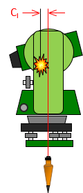 |
| Figure F-16 EM Center |
At the reflector, the EM path slows as it enters the glass and is reflected internally. If the effective distance were plotted as a straight line, the apparent optical center of the reflector would be slightly behind it, Figure F-17. The distance between the optical center and the vertical line through the ground point is CP.
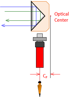 |
| Figure F-17 Reflector Optical Center |
Most holders allow mounting the reflector on the front or back, Figure F-18.
|
|
| Figure F-18 Mount Offsets |
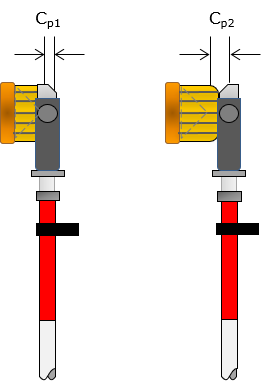
Depending on the side, the reflector is either closer to or further from the EDM/TSI which affects the optical center offset. Contemporary holders generally have the offset value printed on the respective side.
The corrected distance is the sum of the slope distance, EDM/TSI offset, and reflector offset, Figure F-19 and Equation F-4.
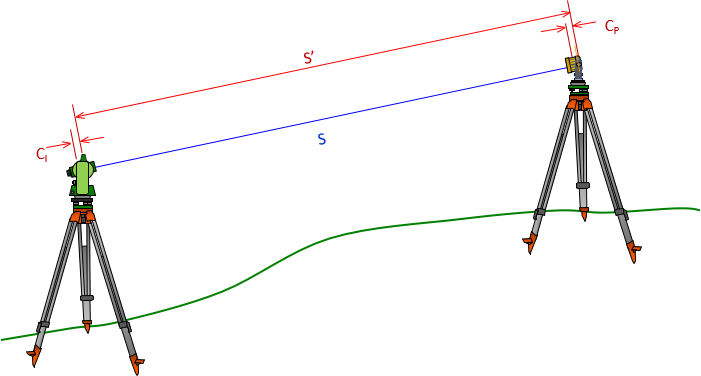 |
| Figure F-19 Measurement Constant |
 |
Equation F-4 |
|
S: corrected slope distance |
|
(b) Behavior
Systematic
(c) Compensation
Procedure: The combined constant should be entered in EDM/TSI prior to measurement. The procedure for determining the combined constant is covered in XV. Equipment Checks and Adjustments Chapter D. Electronic Distance Measurement.
Mathematical: The reflector constant, adjusted for the zenith/vertical angle, should be added/subtracted from the distance. Prior to applying the correction, check if the EDM/TSI has been set with a different constant. If so, adjust the correction accordingly.
(5) Reflector height
(a) Description
For as simple an instrument as is the reflector pole, it can lead to some problems. We have already discussed the pole's bubble; what about its height?
Reflector pole height does not affect horizontal distance determination. Remember that the TSI uses a zenith angle with the slope distance to compute the horizontal distance. Reflector height doesn't matter since raising or lowering it will change both zenith angle and slope distance but still result in the same horizontal distance.
Reflector height can come into play in topographic surveys where elevations are determined trigonometrically using instrument and reflector heights. It behaves systematically. The error and compensation are discussed in IV. Elevations Chapter F. Trigonometric Leveling.
b. Natural
(1) Atmospheric conditions
(a) Description
Electro-optical EM signals are affected by atmospheric pressure and temperature. TSIs are generally standardized at a specific temperature and pressure. When measurement conditions deviate from either then a proportional correction must be applied. This is normally done by the TSI after the operator provides it some necessary information (temperature and pressure or the actual correction factor).
(b) Behavior
Systematic.
(c) Compensation
Procedure: The correction or temperature and pressure are entered in the instrument.
Mathematical: Compute and apply the corrections manually after the fact.
Typical equations for the atmospheric correction are:
| English | ||
 |
Equation F-5 | |
| PE: Pressure, in Hg TE: Temperature; ºF |
||
| Metric | ||
 |
Equation F-6 | |
|
PM: Pressure, mm Hg |
||
Different manufacturers may use slightly different standardization conditions so refer to the user manual for the correction equations for a partucular instrument.
Use Equation F-7 to correct the raw distance.
| D = D'x(1+corr'n) | Equation F-7 |
|
D: Corrected distance |
|
(2) Curvature and refraction
(a) Description
The effects of curvature and refraction on the line of sight are described in II. Errors Chapter E. Systematic Errors. The EDM's EM wave is also bent, affecting horizontal and vertical distances both. Figure F-20 shows the curvature and refraction geometry for distance measurement.
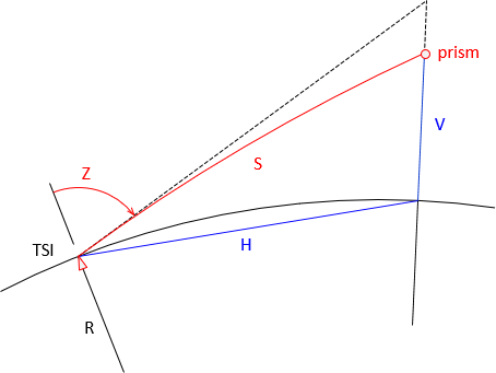 |
| Figure F-20 Slope Reduction, Z<90° |
Red line, S, is the slope distance coincident with the LoS.
The black line is tangent to S at the instrument.
Zenith angle, Z, is measured to the black tangent.
Blue line, H, is the "horizontal" distance.
Blue line, V, is the vertical distance.
In plane surveying, horizontal distance is always shorter than the corresponding slope distance. This isn't the case in geodetic surveying. When the zenith angle exceeds 90°, slope distance is shorter than horizontal, Figure F-21.
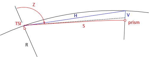 |
| Figure F-21 Slope Reduction, Z Near 90° |
This is demonstrated in the Example Computations section.
(b) Behavior
Systematic
(c) Compensation
Procedure: Modern instruments have the ability to apply refraction and curvature corrections as measurements are made. Data collection software also provide a correction option as does some desktop surveying software. Care must be exercised so that the correction is not applied multiple times. The safest approach is to turn on the correction in the instrument and not in the data collection or desktop software.
Mathematical: Most instrument manuals will describe the algorithms used ti account for curvature and refraction. Equations F-8 and F-9 are examples from one instrument's manual.
|
|
Equation F-8 | |
 |
Equation F-9 | |
| H: Horizontal distance V: Vertical distance S: Slope distance Z: Zenith angle k: refraction constant; low elev: 0.14, high elev: 0.07 R: Earth radius |
||
If the corrections are not applied in the instrument, they can accounted for later.
(3) Atmospheric anomalies
(a) Description
The atmospheric correction and refraction are based on an assumption that the atmosphere is either uniform or changing uniformly along the signal path. This is not always the case. Consider the atmosphere immediately above an asphalt surface on a sunny day - the heat emitted by the surface causes a local atmospheric anomaly which affects the signal path. Almost any surface will have a boundary layer of atmospheric disturbance if it has been subject to sunlight.
(b) Behavior
Random.
(c) Compensation
The effect of atmospheric anomolies can only be minimized or eliminated by not measuring through them. This isn't always practical. For example many Public Land Survey (PLS) corners are located in roads. Not only might the surveyor have to deal with an anomaly at a PLS corner, he may be measuring along the pavement to an adjacent corner half a mile away.
Strategies can include measuring on a cloudy day, late at night, or early morning. Depending on the surface, increasing the TSI and/or reflector height may raise the signal sufficiently above the boundary layer.
a. Personal
(1) Equipment centering
(a) Description
This involves how accurately the operator can center the instrument or tribrach vertically over the ground mark. If using a hand held reflector pole, how carefully the rodperson holds the bubble centered.
(b) Behavior
Random.
(c) Compensation
Practice, practice, practice.
(2) Atmospheric conditions determination
(a) Description
Temperature and barometric pressure must be obtained for the time of measurement.
(b) Behavior
Systematic.
(c) Compensation
If conditions cannot be ascertained in the field, the operator should record the existing settings in the instrument. Conditions at measurement time can be determined from the internet or local radio/TV station later. The measurements can then be "uncorrected" for the recorded field conditions and "re-corrected" using the appropriate data.
8. Example Computations
a. Atmospheric conditions
A distance of 846.39 ft was measured with no atmospheric correction applied by the instrument. What is the corrected distance if the temperature and atmospheric pressure were 85° and 29.2 in Hg?
Using Equation F-5:

Applying the correction with Equation F-7:

b. Slope reduction
The slope distance from a Section corner to a Quarter Section corner was measured as 2648.34 ft at a zenith angle of 92°14'20". What is the effect of earth curvature and refraction on the horizontal reduction?
The last term in Equation F-8 is the curvature and refraction correction for the horizontal distance. Use 14% for refraction and 20,906,000 ft for the earth's radius.
Solving the term for the conditions:

The zenith angle exceeds 90° which makes the correction negative. Because the correction is subtracted, the horizontal distance is actually longer than the slope distance in this situation.
c. Measurement Random Error
A total station's centering error over a point is ±0.005 ft, the reflector is mounted on a pole and its centering error is ±0.02 ft. The MSA for the instrument is ±(3mm + 4ppm). The distance measured is 753.84 ft. What is the expected random error in the distance?
Sketch:
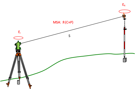
The total random error in the distance comes from the Error of a Sum (refer back to Chapter F. Random Errors):
| Equation F-10 |
The constant and proportional part of the MSA are not independent errors. They are the expected uncertainty in a single measurement. When applying the Error of a Sum, the MSA is treated as a singular error.
| Equation F-11 | ||
|
Ei : Instrument centering error |
||
Compute MSA error components

Use Equation F-11 to determine the expected error.

To further explore random error propagation, check the Distance and Angle Random Error Propagation spreadsheet in the Software section.