K. Reduction Example: SPC
1. Preliminary Calculations
a. Survey Data
This chapter covers measurements reduction for an SPC conic zone. Distances and coordinates will be in survey feet.
The survey data and SPC grid information for point Jerry are summarized in Figure K-1 and Table K-1.
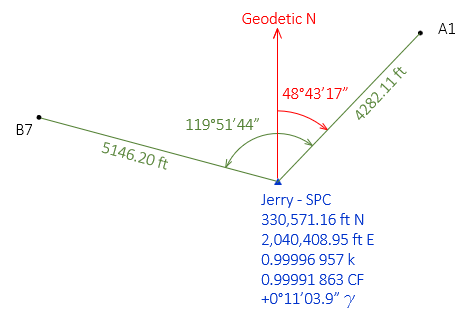 |
| Figure K-1 Survey Data |
|
Table K-1
Orthometric Heights
|
|
| Point |
H, ft |
| Jerry |
1177 |
| A1 |
1805 |
| B7 |
1340 |
b. Approximate Coordinates
Compute approximate SPC coordinates of A1 and B7.
Point A1

Point B7

2. Ground Distance to Grid
a. Ground to Ellipsoid
Going from ground to the ellipsoid is independent of the grid system.
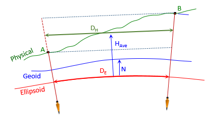 |
| Figure K-2 Ground to Geodetic |
Use Equation H-2 to reduce ground to the ellipsoid
Equation H-2
Te equation uses a line's average elevation and the average geoid height to determine the geodetic length on the ellipsoid.
RE is 20.906 x 106 ft.
Jerry's geoid height is -33.902 meters computed using the GEOID18 model. It is negative because the geoid is below the ellipsoid in Wisconsin.
Since we're working in feet, the geoid height must be converted from meters:

Geoid height generally does not vary significantly over an area of this size. Since Jerry is centrally located, -111.2 ft can be used as a project average.
(1) Geodetic distance Jerry-A1

(2) Geodetic distance Jerry-B7

b. Ellipsoid to Grid
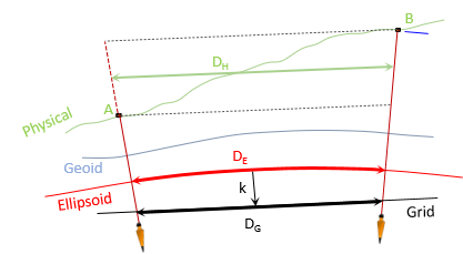 |
| Figure K-3 Geodetic to Grid |
To go from ellipsoid to grid, the geodetic distance multiplied by the grid scale factor, k, Equation H-3.
Equation H-3
The grid scale in Equation H-3 can be:
Jerry's scale used for the entire project
Average of the endpoint scales for each line
A weighted average scale, Equation H-4, for each line based on scales at the mid- and endpoints
Equation H-4
We'll compute the grid distance each way and compare their results.
(1) Using Jerry's scale: k=0.99996 957.
Line
Grid Distance
Jerry-A1: Jerry-B7:
(2) Average scale for each line
Using software, scale at points A1 and B7 can be determined using their approximate coordinates. NGS's NCAT can be used for this as well as the NAD 83 Coordinate Conversion workbook.
| Point |
Scale |
| A1 |
0.99996 8421 |
| B7 |
0.99996 8894 |
Multiplying each line's geodetic distance by its average scale:
| Line |
Average k |
Grid Dist |
| Jerry-A1 |
0.99996 8996 | 4281.768 |
| Jerry-B7 |
0.99996 9232 | 5145.760 |
(3) Weighted average scale for each line
Use the same software to determine the scale at each line's midpoint; midpoint coordinates are the average of the endpoint coordinates.
| Line |
Mid-point k |
| Jerry-A1 |
0.99996 8991 |
| Jerry-B7 |
0.99996 9230 |
Multiplying each line's geodetic length by its weighted average scale:
| Line |
Weighted k |
Grid Dist |
| Jerry-A1 |
0.99996 8992 | 4281.768 |
| Jerry-B7 |
0.99996 9231 | 5145.760 |
(4) Combined Factor
Grid distance can also determined from multiplying ground distance by Jerry's Combined Factor: 0.99991 863, Equation H-6.
| Equation H-6 |
This simplified method does not require computing geodetic distances - the entire project is scaled by a single CF.
| Line |
Grid Dist |
| Jerry-A1 |
|
| Jerry-B7 |
(5) Comparing results
Theoretically, the weighted average scale gives the best grid distance. In Table K-2 it is used as the base to which the others are compared.
| Table K-2 Grid Reduction Comparisons |
||||
| Jerry-A1 | Jerry-B7 | |||
| DE x k |
Grid Dist, ft |
Diff, ft |
Grid Grid, ft |
Diff, ft |
| Wtd Ave k |
4281.768 |
- - |
5145.760 | - - |
| Average k |
4281.768 | 0.000 | 5145.760 | 0.000 |
| Jerry's k |
4281.771 |
+0.003 |
5145.761 |
+0.001 |
| Combined Factor | ||||
| DHxCF |
4281.762 |
-0.006 |
5145.781 | +0.021 |
The largest differences are for the CF grid distances. Considering there is a 255 foot elevation variation across the project, that's not surprising. The other differences are 0.003 ft or less. An acceptable level of accuracy might be achieved with Jerry's scale factor for all lines - it simplifies computations somewhat although using line averages increases the accuracy without too much more effort.
Depending on accuracy requirement, a worse-case scenario should be examined. Consider a line furthest from the control in direction of scale variation and/or at largest elevation difference. Any method acceptable for that line will be acceptable for the entire project.
3. Grid Direction
To convert the geodetic azimuth of line Jerry-A1 to grid, we need to know:
- where the two meridians are with respect to each other, and
- if the arc-to-chord correction should be applied
a. Meridians
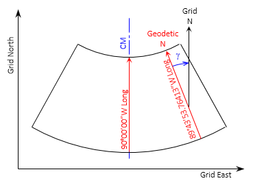
Convergence is the angle from Geodetic N to Grid N. Jerry's SPC convergence is +0°11'03.9". Because it is positive, Geodetic N is west of Grid N, Figure K-4.
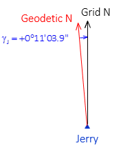 |
| Figure K-4 Geodetic and Grid North |
Another way to determine the meridians' relationship is by comparing longitudes of Jerry and the CM. This requires knowledge of the zone parameters. The CMs of all three Wisconsin SPC zones are at 90°00'00"W longitude. Jerry's longitude is 89°43'53.76413"W which places it east of the CM. Because Jerry is east of the CM, Geodetic N west of Grid N, Figure K-5.
 |
| Figure K-5 Longitudes |
b. Arc-to-Chord
The arc-to-chord correction for line Jerry-A1 can be computed using either Equation H-9 or H-10. We'll use both to see if there's a difference.
 |
Equation H-9 |
 |
Equation H-10 |
Both equations require No which is the north coordinate of the CP at the CM. Even though a constant, it is not given as a zone parameter and must be computed using the projection equations. NCAT does not provide this information but the NAD 83 Coordinate Conversion workbook does.
Wis South SPC Zone No = 510,708.62 ft = 155,664.30 m
(1) Equation H-9
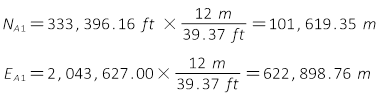
Because Equation H-9 is set up for metric coordinates,we'll need to convert point A1.
Equation H-9 in terms of point identifiers:
Coordinate differences:

Substituting into the correction equation:

(2) Equation H-10
Equation H-10 in terms of point identifiers is:
This coordinates may be metric or Imperial. We'll stick to feet.
This equation requires ro which, like No, is constant for for a zone but not given as a defining parameter. NCAT does not provide this information but the NAD 83 Coordinate Conversion workbook does.
For Wis SPC South zone, ro = 20,920,156.06 ft.
Coordinate differences:

Substituting into the correction equation:

(3) Application
Both equations yield the same result (surprise, surprise).
Is the arc-to-chord correction significant? That's up to the surveyor and the type of project. Even though it's less than a second, we'll apply it as it may affect rounding.
To compute the Grid Azimuth from Geodetic, convergence, and arc-to-chord correction, use Equation H-7.
| Equation H-7 |
A sketch can also be used to determine how to apply the correction. Because the North coordinates of Jerry and A1 are less than No, the line is south of the CP which makes it concave northerly toward the CP, Figure K-6.
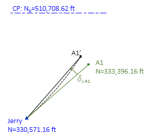 |
| Figure K-6 Line Jerry-A1 Concavity |
The arc-to-chord correction computed with Equations H-9 and H-10 is negative making it an angle to to the left which Figure K-6 supports. Figure K-7 shows all the elements to convert the Geodetic Azimuth to Grid.
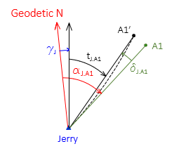 |
| Figure K-7 Grid Azimuth |
Using Jerry's convergence and a negative arc-to-chord correction, the Grid Az of Jerry-A1 is:

4. Ground to Grid Angle
To convert angle B7-Jerry-A1 to grid, we need the arc-to-chord correction for lines Jerry-A1 and Jerry-B7. We have the former, now must compute the latter. Line Jerry-B7 is longer and oriented more east-west than Jerry-A1 so the magnitude of its arc-to-chord correction should to be larger.
We've shown that both arc-to-chord equations give the same results so we'll use Equation H-10.


The correction for Jerry-B7 is larger than Jerry-A1's as expected.
At Jerry the correction to A1 is negative (angle left) and to B7 positive (angle right). The angle and corrections are shown in Figure K-7.
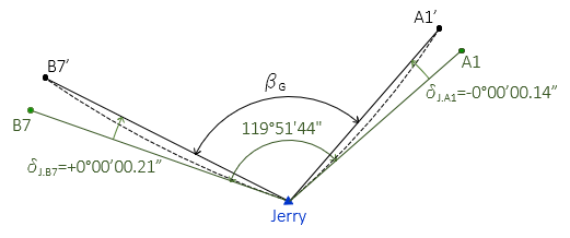 |
| Figure K-7 Angle Corrections |
The grid angle B7'-Jerry-A1', βG , is:

The user must decide if combined bascksight and foresight arc-to-chord correction is significant.
5. Summary
This example looked at a few different SPC grid reduction methods. Depending on the accuracy needs of the survey, simple methods may be sufficient instead of more complicated (and time consuming) ones. The decision should be based on examination of worse-case scenarios.
If the two lines of the example survey represent the extreme situations, we determined that
- distance reduction - Jerry's grid scale could be used for the entire project but each line should use its own average elevation
- arc-to-chord correction - was not significant enough to affect directions or angles.