4. The Danger of Including Mistakes
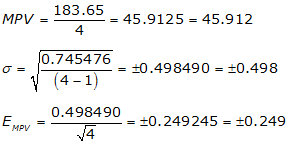
Let’s include a measurement with a mistake and see what happens.
Make the first measurement 46.66, an error of 1.00 units.
num | value | v=meas=MPV | v2 |
1 | 46.66 | 46.66-45.912 = +0.748 | 0.559504 |
2 | 45.66 | 45.66-45.912 = -0.252 | 0.063504 |
3 | 45.68 | 45.68-45.912 = -0.232 | 0.053824 |
4 | 46.65 | 45.65-45.912 = -0.262 | 0.068644 |
sums | 183.65 | 0.745476 |
Note how large the standard deviation and EMPV error become. That’s because both are affected by the huge increase in the residuals caused by pushing parts of the 1.00 unit error into all of them. Including a measurement with a mistake degrades the rest of the measurements.
Always: get rid of mistakes before trying to analyze random errors.
5. What About Unresolved Systematic Errors?
Go back to our mistake-free measurement set: MPV = 45.662 ±0.013; EMPV = ±0.006.
What if these are distances measured with a steel tape and we find out later that the tape started at 1.00' instead of 0.00'? What happens to our analysis?
Well, the MPV changes because each measurement is 1.00' too large (e.g., 45.66 should be 44.66). You can recompute the MPV or just subtract 1.00' from it: MPV = 44.662
How about the standard deviation and MPV error?
They don’t change because the residuals don’t change: since each measurement and the MPV lose 1.00', the residuals stay the same.
But remember that with the systematic error present, the accuracy indivcator (EPMV) is still pretty low which implies good accuracy. An unresolved systematic error will affect accuracy.
So accounting for the systematic error: MPV = 44.662 ±0.013; EMPV=±0.006. That’s the nice thing about systematic errors: you can often eliminate them by computation.