C. Direct Minimization Method
1. General
The most probable value (MPV) estimation of an observation set is the one which that minimizes the sum of the squares of the residuals, Equations C-1 and C-2.
| Equation C-1 | ||
| Equation C-2 | ||
| v: Residual o: Observation |
||
Combining Equations C-1 and C-2 gives Equation C-3; its only unknown is the MPV. To minimize a function, its first derivative is set equal to zero, Equation C-4, and solved for the unknown.
| Equation C-3 | |
| Equation C-4 |
Because the derivative is set to zero, we will refer to this as the Direct Minimization method.
2. Direct Measurement
To demonstrate, determine the MPV of the following set of distance measurements:
| 262.35 |
| 262.40 |
| 262.33 |
| 262.31 |
| 262.38 |
To define the function, set up Equation C-3 for each measurement and add them together:
Take the first derivative of the function, set it equal to zero, and solve for the MPV:

Note that the MPV is the simple average of the observation set.
3. Indirect Measurement Example
For a network with multiple unknowns, minimization requires taking partial derivatives of the function with respect to each unknown and setting them equal to zero, Equation C-5.
 |
Equation C-5 |
If two unknowns are connected by an observation, Equation C-3 will include a residual term containing both unknowns. The partial derivatives will yield a set of simultaneous equations that can be solved for the unknown values.
a. Level Circuit
(1) Original data
Let's revisit the level circuit from Chapter B, Figure C-1.
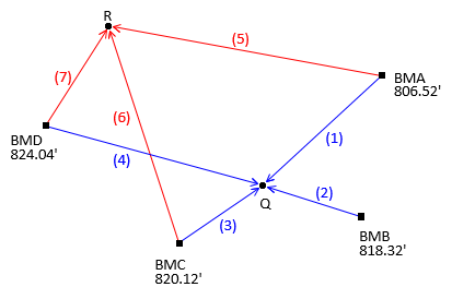 |
| Figure C-1 Level Circuit |
| Obs | Line |
dElev |
Obs | Line |
dElev |
|
| 1 | BMA-Q | +8.91 | 5 | BMA-R | -3.56 | |
| 2 | BMB-Q | -2.92 | -- | -- | ||
| 3 | BMC-Q | -4.67 | 6 | BMC-R | -17.12 | |
| 4 | BMD-Q | -8.66 | 7 | BMD-R | -21.10 |
Create an an observation equation for each elevation difference relating it to the unknown elevation and bench mark. Because these are redundant observations, each equation contains a residual. Equation C-6 is the initial observation equation format, then rearraged to place the residual on the left side, Equation C-7.

Equation C-6 
Equation C-7
For Observation 1:

The seven observation equations are:

The residuals are substituted into Equation C-3:
![]()
Because there aren't any observations directly linking points Q and R, they do not appear together in any of the residuals.
We can take the derivative of the function with respect to each elevation and determine its elevation separately.


These are the same elevations determined by the Brute Force method. Surprised?
The Standard Deviation of Unit Weight, So, would be computed using the residual observation equations and Equation A-6.
(2) Added Observation
How is an eighth observation connecting points Q and R, Figure C-2, incorporated?
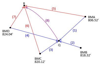 |
| Figure C-2 Added Observation |
dElev(8) = -12.47
Each observation adds a residual term:

Notice that the added residual contains both unknown elevations.
The term is added to function, F:
Take partial derivatives of the function with respect to each elevation and set equal to zero:


The result is two simultaneous equations. Solve using either Substitution or Gaussian Elimination.
Using Substitution
| Solve the first partial in terms of ER | |
 |
Substitute into the second partial. Solve elevation of point Q |
| Substitute EQ back into first equation to determine elevation of point R |
The elevations of points Q and R change slightly from the previous adjustment. Because they change and the number of observations increased, So must be recomputed.
Use the eight observation equations to compute the residuals.

(3) Adding More Observations
To add a ninth observation, dElev(9)=+12.44, from point R to point Q, Figure C-3...
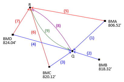 |
| Figure C-3 Another Observation Added |
...create another observation equation:

Add the residual term to function F, take partial derivatives with respect to ER and EQ, and solve as before. The same process is followed for any additional observations. Regardless how many unknowns and observations, Figure C-4, there are never more than two unknowns in each residual term.
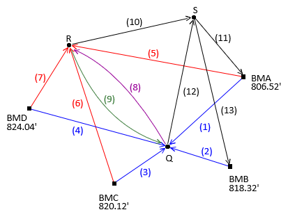 |
| Figure C-4 More Observations |
Although the network in Figure C-4 has 10 DF, only three equations are solved simultaneously for the LS adjustment.
4. Chapter Summary
Unlike the Brute Force approach, Direct Minimization does not require determining each possible elevation before computing averages. This method requires only that appropriate observation equations are constructed and partial derivatives taken with respect to each unknown. It's more flexible than Brute Force, but can still be improved on. For example, determining uncertainties for adjusted values and observations is, frankly, a pain. Fortunately, there's a systematic approach that addresses deficiencies of Brute Force and Direct Minimization.