{KomentoDisable}
H. Ground to Grid Conversion
1. Grid Distances
a. General
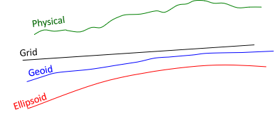
In the Horizontal Datum topic, we defined three Earth surfaces and their height relationships, Figure H-1.
 |
| Figure H-1 Surfaces and Heights
|
Adding a grid introduces another surface, Figure H-2.
 |
| Figure H-2 Inserting a Grid Surface |
To convert a ground distance to grid, Figure H-3, requires going from the horizontal measurement on the physical earth, DH, to the ellipsoid, DE, then to the grid, DG.
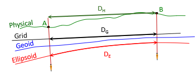 |
| Figure H-3 Ground Distance to Grid Distance |
DE is a geodetic distance since it is on the ellipsoid's surface.
b. Ground to Ellipsoid
Going from ground to the ellipsoid, Figure H-4, is done using a proportion, Equation H-1.
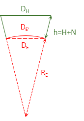 |
| Figure H-4 Ground to Ellipsoid |
 |
Equation H-1 |
RE is the ellipsoid radius. The ellipsoid has different radii depending on a line's direction and location. Because a survey line covers such a small part of the ellipsoid, its radius can be assumed constant. 6,372,200 m or 20,609,000 ft is typically used for RE. Section 3 discusses discusses different radii and their effect on distance reduction.
The ground distance, DH, is a straight line so DE computed from Equation H-1 is a chord. The geodetic distance should be along the ellipsoid's surface, DE'. The difference between the two isn't significant: the chord distance for a 20,000.0000 ft geodetic distance is 19,999.9992 ft. The distance from Equation H-1 can be used directly as the geodetic distance.
If there is a significant elevation difference between ground points and they are far enough apart, the horizontal distance between them differs based on which point it is referenced to. In Figure H-5, the distance at point B's elevation is longer than it is at point A's.
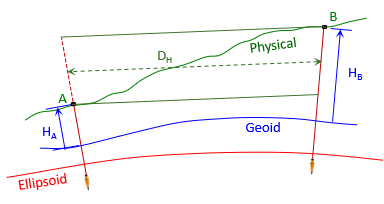 |
| Figure H-5 Average Elevation |
To reduce the distance to the ellipsoid, the line's average elevation is used so Equation H-1 is modified to Equation H-2.
 |
Equation H-2 |
The term inside the brackets is called the Elevation Factor, EF, since it accounts for the orthometric and geoid heights.
The geoid doesn't vary much over a line's length so the geoid height at either end, or an average, can be used. Geoid heights over larger areas can be determined using NGS's GEOID18 Computation Tool.
The geodetic distance is independent of the grid system projection. The projection only matters when going from the ellipsoid to the grid.
c. Ellipsoid to Grid
The geodetic distance is multiplied by the scale factor to obtain the grid distance, Equation H-3.
| Equation H-3 |
k - scale factor (aka, grid scale)
Scale is a function of the grid system location, as discussed in Chapter D. It is either computed using projection equations or obtained from the grid attributes at a control station. The latter is covered in Chapter I.
For short lines, the grid scale at either end can be used. Where the scales different significantly, their average, or weighted average (Simpson's Rule), Equation H-4, can be used.
| Equation H-4 |
Because the ellipsoid isn't spherical, midpoint scale, km, is not the average of the scales at both its ends.
d. Combined Factor
The Elevation Factor and scale can be multiplied to create the Combined Factor, CF, Equation H-5. Each ground distance can be multiplied by the CF to go directly to grid, Equation H6.
 |
Equation H-5 |
| Equation H-6 |
Because they use average values, Equations H-5 and H-6 work best over smaller project areas where elevation changes are not excessive.
2. Grid Directions and Angles
a. Convergence Angle
The angle from Geodetic North to Grid North is the Convergence, γ. In NAD 27 systems, it was called the mapping angle. Along the CM, Geodetic and Grid North coincide so there is no convergence. Convergence magnitude increases with distance east or west from the CM.
On a conic projection, Figure H-7, geodetic meridians (red) converge to the North Pole.
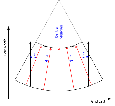 |
| Figure H-7 Conic Convergence |
The geodetic meridians on a transverse cylinder are more complex. On the grid they are curved lines converging to the North Pole, Figure H-8. The closer to the pole, the greater their curvature.
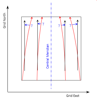 |
| Figure H-8 Cylindric Convergence |
Convergence is positive (+) east of the CM, negative (-) west, Figure H-9.
 |
| Figure H-9 Math Sign |
b.Projected lines
A geodetic line on the ellipsoid doesn't project as a perfectly straight line on the grid but is slightly curved. The curvature amount depends on the line's orientation. On a conic projection, Figure H-10(a), it is most pronounced for east-west lines and is concave toward the Central Parallel. On a transverse cylindric projection, the curvature is largest for north-south lines, Figure H-10(b), and is concave toward the Central Meridian.
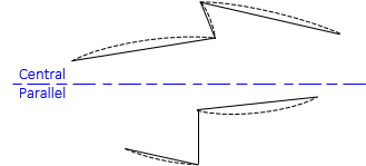 |
| (a) Conic Projection |
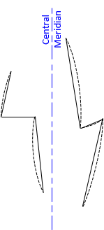 |
| (b) Transverse Cylindric Projection |
| Figure H-10 Projected Lines |
Geodetic meridians, being geodetic lines, also project slightly curved Figure H-11 shows a highly exaggerated depiction of the angle and direction relationships between straight and projected lines.
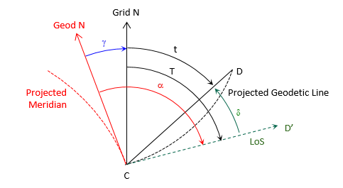 |
| Figure H-11 Projected Line Relationships |
Geodetic north (solid red) on the grid is tangent to the projected meridian (dashed red) at the user's position, point C. When the observer sights point D, his line of sight (dashed green) is tangent to the projected line CD (dashed black). The angle between the line of sight and the straight chord CD is the arc-to-chord correction, δ.
Other elements in Figure H-11 are
T - grid azimuth of the projected line of sight
t - grid azimuth of the chord
α - geodetic azimuth of the projected line of sight
Equations H-7 and H-8 are the relationships between the various angles and azimuths.
| Equation H-7 | |
| Equation H-8 |
The arc-to-chord correction is also called the second term or (t-T) correction.
Equations H-9 and H-10 are arc-to-chord correction equations for conic projections.
 |
Equation H-9 |
 |
Equation H-10 |
Either can be used although Equation H-9 is set up for metric units.
Equations H-11 and H-12 are for transverse cylindric projections.
 |
Equation H-11 |
 |
Equation H-12 |
Either can be used although Equation H-11 is set up for metric units.
In the equations:
| δ12 | Correction for line 1 to 2; seconds |
| N1, E1 | Coordinates of from point 1 |
| N2, E2 | Coordinates of to point 2 |
| No | Northing at intersection of CM and Central Parallel |
| ro | Mean radius at origin latitude |
| Eo | CM Easting |
The Central Parallel of a conic projection is not the same as the Origin Parallel nor is it midway between North and South Standard Parallels. Its northing, No, is a constant but it must be computed from a zone's parameters.
Approximate coordinates can be used for both points in all four equations.
The mathematical sign on the correction indicates its direction: positive (+) is an angle to the right, negative (-) is an angle to the left.
If arc-to-chord corrections are significant they should be applied to the backsight and foresight lines of measured horizontal angles, Figure H-12, using Equation H-13,
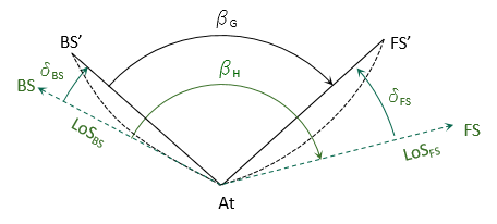 |
| Figure H-12 Corrected Angle |
 |
Equation H-13 |
where:
| βH | measured horizontal angle |
| βG | grid angle |
| δBS | backsight arc-to-chord correction |
| δFS | foresight arc-to-chord correction |
For most surveys,the corrections are generally smaller than angle measurement accuracy. To determine if they should be applied, compute the angle correction for a survey's the worst-case scenario; if it isn't significant, they can be ignored for all the angles. If that's the case, Equation H-7 becomes:
| Equation H-14 |
c. Forward and Back Directions
Because grid meridians are parallel, the forward and back grid azimuth of a line, Figure H-13, differ by exactly 180°, Equation H-15.
 |
| Figure H-13 Forward and Back Grid Azimuths |
| Equation H-15 |
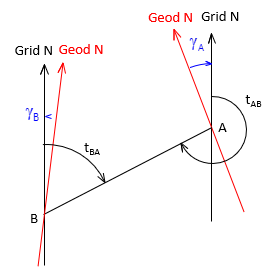
The line's forward and back geodetic azimuths, Figure H-14 , must account for the convergence difference at each end, Equation H-16.
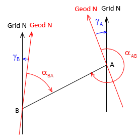 |
| Figure H-14 Forward and Back Geodetic Azimuths |
 |
Equation H-16 |
3. Ellipsoidal Radii
Equation H-1 requires a radius to reduce ground distance to geodetic. Because the ellipsoid is not a sphere, it does not have a single uniform radius. At each point on the ellipsoid, there are (at least) three different radii. These are dependent on the point's ellipsoid location.
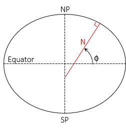
a. Normal, N
The normal is the line perpendicular to the ellipsoid surface at the observer's position, Figure H-15.
 |
| Figure H-15 Normal |
It is in the observer's meridian and extends to the semi-minor (polar) axis. The angle from the semi-major axis to the normal is the geodetic latitude, Φ.
The length of the normal varies between a at 0° lat and b at ±90° lat, Equation H-17
 |
Equation H-17 |
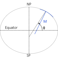
b. Meridional Radius, M
The shorter an ellipsoidal arc segment, the closer it comes to being a circular arc. The meridional radius, M, is the radius of an infinitesimally short arc in the meridian at the observer's position, Figure H-16.
 |
| Figure H-16 Radius in Meridian |
Like the Normal, its length depends on geodetic latitude, Equation H-18.
 |
Equation H-18 |
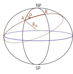
c. Radius in an Azimuth, Rα
A meridian is an ellipse with the same semi-major and -minor axes as the reference ellipsoid. Connecting two points A and B not in the same meridian will create a new ellipse. If the points are at
- the same latitude, the ellipse will be at a 90° azimuth to A's and B's meridians and form a circle of fixed radius.
- different latitudes, the ellipse will be at an azimuth other than 90° (or 270°) and have semi-major and -minor axes different than the reference ellipsoid.
The radius in the direction of line AB is similar to a meridional radius except it is for a section along the new ellipse, Figure H-17 and Equations H-19 and H-20.
 |
| Figure H-17 Radius in an Azimuth |
| Equation H-19 | |
 |
Equation H-20 |
d. Radius RE?
RE is typically 20,906,000 ft or 6,372,200 m which is a mean value and not dependent on latitude or direction. How does geodetic reduction using this radius compare to the others?
An example can be used to illustrate. Given:
- Latitude of point A is 41°30'00"
- Azimuth and distance to point B are 55°45'00" N and 10,000.00 ft.
- Elevations of points A and B are 900.0 ft and 800.0 ft
- Area geoid height is -32.0 m
- GRS 80 ellipsoid a = 6,378,137.0 m, e = 0.08181 919104, e' = 0.08209 44382
Compute the radii


Compare to RE = 20,906,000 ft
| Radius |
Value |
diff |
diff |
| RE |
20,906,000 ft | - - | - - |
| N | 20,956,425.4 ft | +50,425.4 ft | +0.24% |
| M |
20,877,499.8 ft | -28,500.2 ft. | -0.14% |
|
Rα |
20,931,361.3 ft | +25,361.3 ft | +0.12% |
Those seem like substantial differences. How do they affect distance reduction to ellipsoid? Use each in Equation H-1 to determine the geodetic length of line AB and compare them to using RE.
| Radius |
DE |
diff |
| RE |
9,9999.6436 ft | - - |
| N | 9,9999.6445 ft | +0.0009 ft |
| M |
9,9999.6432 ft | -0.0004 ft |
| Rα | 9,9999.6441 ft | +0.0005 ft |
Despite the large radii variation, there is no significant effect on distance reduction. Even with a ground distance of 20,000 ft, the maximum difference is only 0.002 ft.
This basic analysis shows that 20,906,000 ft can be used for grid to geodetic distance reduction without affecting accuracy.
4. Reduction Summary
If it seems like there are a lot of computations involved, well, there can be. Measurements are distorted going from ground to grid and these computations are used minimize their impact.
Depending on the project scope or accuracy needs, some generalizations can be made to reduce computations. For example, it may be possible to use a single Combined Factor for distance reductions or arc-to-chord corrections may be small enough to ignore. On the other hand, a control quality survey may require each line and direction be individually reduced.
Computations can also flow in the other direction: grid to ground. These are largely a reversal of the of the procedures described in this chapter and might be generalized based on project needs.