{KomentoDisable}
G. State Plane Coordinates
1. General
The State Plane Coordinate (SPC) System has its origin in 1930's when the then named U.S. Coast and Geodetic Survey (C&GS) created a state-wide grid system for North Carolina using a conformal conic projection. Soon thereafter, C&GS created one or more zones for each state. Depending on physical configuration, a conic or transverse cylindric projection, or a combination, was used.The lone exception was the Alaska panhandle which used an oblique cylindric projection. Projections were conformal to preserve angular relationships.
Figure G-1 shows the original SPC zones developed for NAD27 and based on the Clarke 1866 ellipsoid.
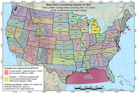 |
| Figure G-1 NAD 27 State Plane Coordinate Zones source: geodesy.noaa.gov/SPCS/maps.shtml |
Michigan actually had two sets of state plane coordinate systems: One using three conic projections and a second using three transverse cylindric. The conic projections were fit to an elevation 800 feet above sea level (and consequently the Clarke 1866 ellipsoid because there was no separation between geoid and ellipsoid for NAD 27). This was done to eliminate the ground to ellipsoid reduction since most of Michigan was within 200 feet of 800 ft elevation. Refer to Special Publication 65-3 Plane Coordinate Projection Tables Michigan, available in the NGS Publications Library.
When the NAD 83 horizontal datum was redefined and readjusted, SPC zones were re-referenced to the GRS 80 ellipsoid. Most zones stayed the same although there were some aggregation, Figure G-2.
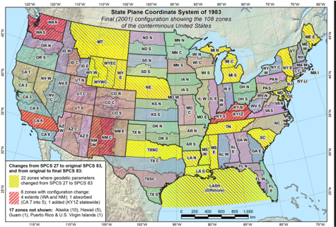 |
| Figure G-2 NAD 83 State Plane Coordinate Zones source: geodesy.noaa.gov/SPCS/maps.shtml |
2. Projection Parameters
Projection parameters are in these publications area on the NGS website:
- SPC 27 - Special Publication 62-4 State Plane Coordinates by Automatic Data Processing
- SPC 83 - NOAA Manual NOS NGS 5 State Plane Coordinate Systems of 1983
These publications also contain equations for converting between geodetic and state plane coordinates, grid scale calculation, and determining the arc-to-chord correction.
3. Jurisdictional Boundaries
Even though zones are based on mathematical projections,their boundaries generally coincide with counties or parishes. For example, Wisconsin uses three conic-base zones: South, Central, and North. Figure G-3 shows these zones overlaid on a map of the counties.
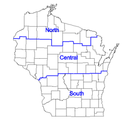 |
| Figure G-3 Wisconsin SPC Zones and Counties |
While C&GS/NGS mathematically designed the zones, states decided their jurisdiction limits. Keeping counties or parishes entirely within a single zone supported uniform surveying and mapping activities. This became increasingly important with adoption of geographic information systems at local jurisdictional levels.
4. Distortion
The maximum ellipsoid to grid distortion for SPC 27 was 1/10,000. This limited individual zone extents to around 160 miles necessitating multiple zones in most states. At the time of their original design, 1/10,000 was considered sufficient as most surveys (done with tape and transit) were below that standard.
By time of NAD 83 adoption, typical surveying accuracy easily exceeded 1/10,000 and because distortion is systematic, some states combined multiple SPC 27 zones into fewer SPC 83 zones. Although 1/10,000 was still a nominal design standard for SPC 83, it became less of an issue.
5. Software
NGS Coordinate Conversion and Transformation Tool (NCAT) is an online package for performing coordinate conversion, and computes convergence and grid scale factor. Input and output can be interactive or file-based.
There's also a simple NAD 83 Coordinate Conversion Excel workbook I put together. It includes all the SPC zones (except Alaska) and UTM zones which cover the US. The workbook is handy If you're interested in the mathematics of conversions. Click here to download it.
I put together a summary document of NAD 83 SPC equations and parameters for CONUS. It can be downloaded from this link.