{KomentoDisable}
C. Solving Equations
1. Linear Equations
a. The Straight and Narrow
A linear equation is a straight line in two or more dimensions. A single equation consists of coefficients, variables, and a constant. In the equation 1.5x-4.5y = 25
x and y are variables.
1.5 and -4.5 are coefficients, numeric values by which the variables are multiplied.
25 is a constant, the result of applying the coefficients to specific variable values.
In a single equation with two variables, assigning a value to either variable defines the other. If both are unknown, the equation cannot be uniquely solved because there are an infinite number of value combinations for x and y that satisfy the equation.
Values of the same two variables in two different linear equations can be determined, providing the equations do not represent parallel lines. There is a single set of values which satisfy both equations at the same time. In graphic terms, x and y are coordinates where both lines intersect.
![]()
We could solve these equations graphically by plotting both and interpolating their intersection’s coordinates, Figure C-1.
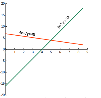 |
| Figure C-1 Plotted Equations |
Accuracy is limited by our graphing and interpolation abilities
b. Numeric Solution
The coordinates can be determined with greater accuracy from the equations. There are several ways to do this, two of which are Substitution and Gaussian Elimination.
(1) Substitution
Rearrange the first equation in terms of y.
![]()
Substitute it into the second equation and solve for x.
![]()
(2) Gaussian Elimination
One equation is multiplied or divided by a constant, then added to or subtracted from another equation to eliminate one of the variables. The more variables, the more times this is done, creating intermediate equations with fewer variables until there is a single equation in a single variable. The variable is solved and then substituted back into intermediate equations until all variables are solved. It sounds more complicated than it is.
In this case, multiply the second equation by 2, subtract from the first. This eliminates x and leaves a single equation in terms of y. Solve y.

Then substitute y into either equation to solve x.
Neither way is particularly difficult, but as the number of equations and unknowns increase (3 equations in 3 unknowns, 4 in 4, etc), the math involved increases accordingly.
Solving simultaneous linear equations is relatively straightforward: their geometry is simple and there is just one intersection point. The only condition the two equations must meet is that they cannot represent parallel lines.
2. Non-Linear Equations
a. Bend Me, Shape Me
Solving non-linear equations is a bit more difficult. Consider the following two equations:

Values for x and y can't be determined by Substitution or Gaussian Elimination. Both are second degree polynomials: each is a curve with a single inflection point. Increasing a polynomial's degree introduces more inflection points complicating conditions even further. Adding trig functions can add insult to injury.
We could plot the curves and pick their intersection graphically, Figure C-2.
|
|
|
Figure C-2 |
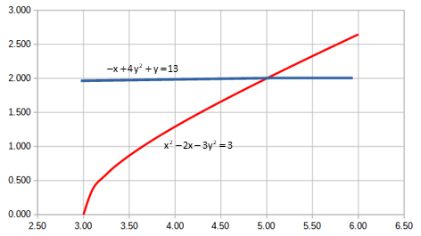
But that can be tedious and limit accuracy to below that desired. Notice how flat -x+4y2+y=13 plots: almost a straight line, but not quite. A plotting error in that curve can substantially affect its intersection with the second line.
A numeric solution is preferred. One simplified way to solve simultaneous non-linear equations is a Taylor Series.
b. Taylor Series
(1) Derivatives
A Taylor Series determines an equation's root by stating with an initial approximation (an educated guess) which is refined with a series of corrections. The corrections are based on successive partial derivatives of the equation.
In general, for any non-linear function in a single unknown B(x), its root is determined from:

The greater the value of n, the better the solution; n = infinity being the best (theoretically).
(2) Iterative Solution
Because not all functions can be derived to infinity (nor would it be prudent time-wise), a practical approach is to drop everything after the first derivative. The first partial is the largest contributor with each successive derivative substantially smaller. Using an initial approximation for the variable, xo, the abbreviated series is used to compute a correction, dx.

The correction is applied to xo and the series solved again generating another update. This iterative process continues until, theoretically, dx is zero. Because of the approximate nature of the abbreviated series, it could take an infinite number of iterations to achieve exactly dx=0.
Instead, iterations continue until an acceptable cutoff for dx is met. For example, if the answer must be good to 0.01, iterations may stop after dx=±0.005 ft. The better the initial approximation, xo, the more quickly the solution will converge.
The non-linear equation must have at least one real root.
x2-2x+3=0 cannot be solved with a Taylor Series because both its roots are imaginary.

Where multiple real roots exist, the Taylor Series will converge to one closest to the initial approximation.
(3) Example
Using a Taylor Series, determine a root to nearest 0.001 for the expression F(x) = x2-9x+2=0
The derivative of the equation with respect to x is:
Set up the Taylor’s Series and rearrange the equation to solve for dx:

Starting with an initial approximation of 1, compute dx:

Update the initial approximation and compute a new dx:

Update and solve again:

...until the difference is small enough for the iterative solution to terminate. In this case, 0.001 meets our criterion, so with one last update we're done:
Solution: x=0.227+.0001=0.228
Because this is a second degree polynomial, it should have a second root. Starting with xo= 10, the Taylor Series converges to x = 8.77.
Check with a quadratic solution:

Figure C-3 is a graphic plot of the equation showing where the equation crosses y=0.
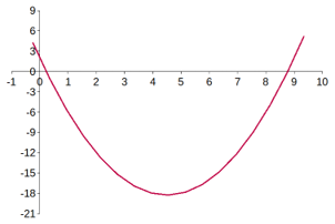 |
| Figure C-3 F(x) = x2-9x+2=0 |
(4) Higher Degrees
So why use a Taylor Series if the equation can be solved with the quadratic solution? Because the quadratic solution is for a second degree polynomial. Higher degrees are much less likely to be easily solved. The quadratic solution cannot determine the roots of 4x3-x2+3x = 34, but a Taylor Series can.
c. Two Variables
(1) Multiple Derivatives
When applied to a single equation with a single variable, a Taylor Series will find the equation roots, the values where the function is zero. When applied to two simultaneous non-linear equations in two variables, the Taylor Series determines their intersection point(s).
To solve two non-linear equations:

we apply a Taylor Series to both simultaneously. Partial derivatives, from i=1 to n, for each variable are added to the function evaluated at initial approximations for both unknowns.
The Taylor Series for two equations in two unknowns, D(x,y) and E(x,y), are:


Each derivative is a correction applied to some initial approximations.
As with a single variable equation, the Taylor Series approximation includes just the first derivative for each variable.
The truncated Taylor Series results in two equations in two unknowns: dx and dy. These are corrections to the initial approximations, xo and yo. Using the iterative approach, initial approximations are updated, new corrections computed, and the process repeated until some threshold level for corrections is reached.
(2) Example 1
Determine x and y for the following equations using a Taylor Series.

Partial derivatives for both equations with respect to each variable are:


Starting with xo=4 and yo=3

Solving the two simultaneous equations results in dx = +1.167 and dy = -0.833
Update x and y and solve again; second iteration:

And so on...
| Third iteration | Fourth iteration | |||
| x | 5.029 | x | 5.000 | |
| y | 2.203 | y | 2.000 | |
| dx | -0.029 | dx | 0.000 | |
| dy | -0.023 | dy | 0.000 | |
The solution converges in four iterations, three if ±0.05 is sufficiently accurate.
Final answers: X=5.0, Y=2.0
(3) Example 2
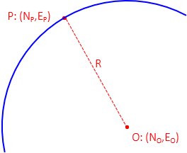
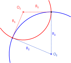
The equation of a circle is N2+E2 = R2 where N and E are the radius point coordinates. If we have coordinates of the radius point and another on the perimeter, Figure C-4, the radius can be computed from:
![]()
|
|
|
Figure C-4 |
In coordinate geometry (COGO), we often need coordinates at the intersection of two circular arcs. Using the radius point coordinates and radii, equations can be written for both circles and their intersection, Figure C-5.
 |
|
|
Figure C-5 |
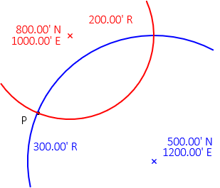
Because they are non-linear equations, a Taylor Series can be used to solve NP and EP. The equations are second degree polynomials so there are two possible intersection points. Initial approximations should be selected which are closer to the desired intersection than the other.
Given the data in Figure C-6, what are the coordinates of point P?
|
|
The closer the initial approximations are to point P, the quicker the solution will converge. We will start with 600.00’ N and 900.00’ E. |
|
Figure C-6 |
Using function A to represent one circle and B the other, the two equations can be written as:
![]()
![]()
Partial derivatives of each equation with respect to NP and EP are:


Set up the Taylor Series approximations with initial coordinate approximations.


Substitute dN from function A into function B.

Then substitute dE back into dN.
![]()
Apply the corrections to the initial approximations.

Re-solve the Taylor Series with the updated coordinates:


![]()
The corrections are still relatively large, so update the coordinates and repeat.

| dN | dE | updated N | updated E |
| +0.05 | +0.02 | 615.38 | 923.08 |
| +0.002 | +0.003 | 615.38 | 923.08 |
Final coordinates: NP = 615.38, EP = 923.08
3. Summary
In surveying we have linear and non-linear mathematical relationships. Examples of both are:
• Differential leveling. Elevations are determined by addition and subtraction which are simple linear relationships.
• Traversing. Horizontal positions are determined by applying non-linear trigonometric functions to distances and angles.
If the number of variables is reasonably small and the mathematical relationships simple, “long-hand” solutions aren’t overly difficult nor time consuming. Three or more variables and non-linear mathematics increases computations along with error opportunity as demonstrated by the circle-circle intersection example. There are two ways to address this.
a. Systematic solution method
The Substitution and Gaussian Elimination methods require the user make decisions how to proceed step-by-step. Although each person may ultimately arrive at the correct solution(s), not all will follow the same solution process. A systematic method is efficient, repeatable, and applicable to multiple situations.
b. Replace the person with software
Almost any computation is quicker using software than paper and pencil. Software still needs a person who understands how to set up data and interpret results. Software can be simple, acting like a high speed calculator, or complex, providing greater flexibility. Because a computer can not “think” in the conventional sense, software must be based on a systematic solution method.
The former will be discussed in greater detail in later chapters along with general comments on software tools.