{KomentoDisable}
H. More Horizontal Examples
1. Distance Intersection
Distance intersection, also known as Trilateration, is used to determine the position of an unknown point from two or more control points. Two control points with a distance from each intersect at two possible locations. Adding a third control point and distance eliminates one of the intersections. The presence of random errors, however, means the three distances will not intersect perfectly.
Figure H-1 is shows three control points with distances that intersect at point P. Use a least squares adjustment to determine the best coordinates of point P, its uncertainty, and error ellipse.
 |
| Figure H-1 Distance Intersections |
Initial coordinate approximations for point P
Distance and azimuth of line BA:

Law of Cosines to solve angle at B from A to P

Compute azimuth from B to P

Forward computation from B to P

Calculate initial distances using point P's initial approximate coordinates
Because point B was used to compute point C, the computed distance is the measured distance.

Perform inverse computation to obtain distances from points A and C


Matrix structures

Set up the observation equations
Dist AP

Dist BP

Dist CP

Set up matrices

Solve the matrix algorithm iteratively

First iteration


Invert the [CTC] matrix using Determinant Method

Compute coordinate updates

Update point P's coordinates

Second iteration
Update [C] and [K] matrices using the observation equations and new coordinates of point P.

Recompute updates

Solution converged.
Adjusted distances
Compute distance residuals from

Since the last updates were zero, [C x U] is a column matrix with all elements equal to zero. Therefore:

Adjusted distances

Position uncertainties


Compute error ellipse


The error ellipses in Figure H-2 are magnified 25 times since they would not be visible at the drawing scale.
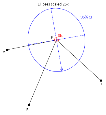 |
| Figure H-2 Standard and 95% CI Error Ellipses |
Adjustment Summary
| NP = 2530.024' ±0.574' | EP = 1109.762' ±0.519' | |
| Error Ellipse | ||
| AzU = 170°04' | ||
| SU = ±0.576' | SV = ±0.517' | |
| SU 95% = ±8.14' | SV 95% = ±7.30' | |
2. Triangulation
A triangulation network is a survey composed of primarily angle measurements. Before electronic distance measurement, most control surveys were done with triangulation since it was faster to measure angles than distances. Triangulation networks required periodic distances, called baselines, to help fix geometry. But a point position can be fixed with just angle measurements for an intersection like in Figure H-3.
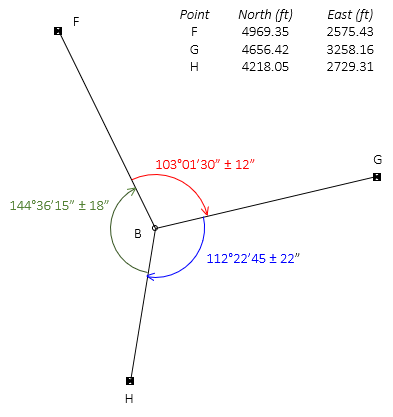 |
| Figure H-3 Intersection by Angles |
The survey has three measurements and two unknowns so a least squares adjustment can be used to determine point B's coordinates.
Point B initial coordinates
There isn't sufficient information to easily compute coordinates for point B (try it, you'll see). But because the adjustment is iterative, we just need reasonable coordinate values to start with. The better the initial values, the fewer iterations needed.
We'll guesstimate coordinates based on point B's proximity to the others. Point B is approximately one third the distance north from point H to point F and approximately one quarter the distance east from point F to point G:

Matrix Structures
Because each angle has an uncertainty, a weight matrix will be used.

Set up observations
General angle observation equation: F-From, A-At, T-To

Since point B is the At point for all three angles, only the third and fourth terms of the observation equation are computed.
Compute distances

Angle FBG


Angle GBH


Angle HBF


Set up matrices

[K] matrix values are large due to point B's guesstimated coordinates. If they are too far off, the solution might not converge. Let's see what happens.
Solve the matrix algorithm iteratively
![]()
First iteration

Coordinate corrections are relatively large, a reflection of our guesstimated point B coordinates.
Updated coordinates are: NB1 = 4,556.558 EB1 = 2,779.278
Second iteration
Recomputed matrices

Corrections are getting smaller - going in the right direction. All right!
Updated coordinates are: NB2 = 4,545.909 EB2 = 2,783.113
Third iteration

Now we're cooking - corrections are smaller. One more should do it.
Updated coordinates are: NB3 = 4,545.954 EB3 = 2,782.940
Fourth iteration

Bingo! The solution took four iterations because our initial coordinates for point B were pretty rough. A better guesstimate might have reduced the iterations to three or possibly two. Worse approximations might have increased the iterations or possibly caused the solution to diverge.
Final coordinates: NB = 4,545.954 EB = 2,782.940
Adjusted Angles
Because the final corrections are 0.000, the angle residuals are the last computed [K] matrix values.

Position uncertainties


Compute standard and 95% CI error ellipses


The standard and 95% CI error ellipses are shown in Figure H-4.
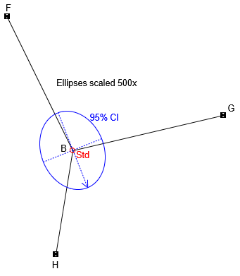 |
| Figure H-4 Standard and 95% CI Error Ellipses |
Because the ellipses are much smaller than those in the trilateration example, they must be magnified considerably more (500x) in order to be seen.
Adjustment Summary
| NB = 4,545.954' ±0.018' | EB = 2,782.940' ±0.014' | |
| Error Ellipse | ||
| AzU = 158°22' | ||
| SU = ±0.018' | SV = ±0.014' | |
| SU 95% = ±0.254' | SV 95% = ±0.198' | |