{KomentoDisable}
G. Error Ellipses
1. Introduction
Each adjusted position has uncertainty based on measurement random errors. A single dimension elevation has a vertical uncertainty, ±SElevP, Figure G-1.
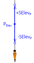 |
| Figure G-1 Elevation Uncertainty |
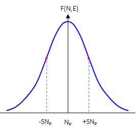
Recall that the standard deviation of a normal distribution is approximately 68% under the symmetric bell-shaped distribution curve, Figure G-2.
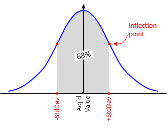 |
| Figure G-2 Normal Distribution |
Standard deviation represents a 68% confidence interval. In Figure G-1, we have a 68% confidence the "true" elevation is within ±SElevP of the adjusted value ElevP.
A two dimension horizontal position has two uncertainties: one north, SNP, one east, SEP, Figure G-3.
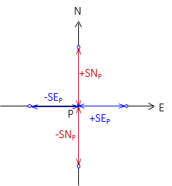 |
| Figure G-3 Horizontal Uncertainties |
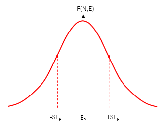
A horizontal position has two normal distribution curves, Figure G-4, corresponding to each direction.
 |
 |
| (a) North | (b) East |
| Figure G-4 Horizontal Position Normal Curves |
|
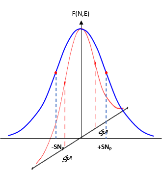
Even though each direction can have a different standard deviation, the two distributions are dependent on each other. They are related by the two dimensional measurements that define the position. Instead of a single simple normal distribution, the expected positional error is a bivariate normal distribution. Combining both curves, Figure G-5, creates the three dimensional bivariate distribution.
 |
| Figure G-5 Bivaraiate Distribution |
The perimeter trace of horizontal "slice" through the bivariate distribution is an ellipse, Figure G-6.
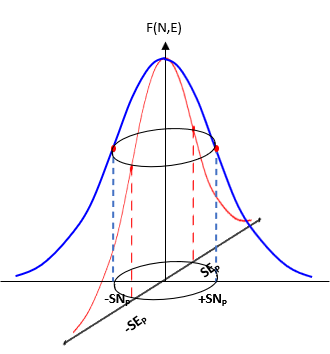 |
| Figure G-6 Error Ellipse |
There are an infinite number of error ellipses, each representing a confidence region centered on the adjusted position. The standard error ellipse is the defined by the standard deviations in the North and East directions.
2. Standard Error Ellipse
a. Defining the Ellipse
An adjusted point's error rectangle, Figure G-7, can be defined by the North and East uncertainties.
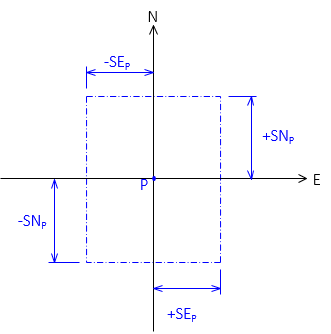 |
| Figure G-7 Error Rectangle |
An error ellipse is tangent to all four sides of the error rectangle. If North and East uncertainties are the same, the error ellipse would be a circle. With differing uncertainties, there are infinite ellipses tangent to the error rectangle sides, Figure G-8.
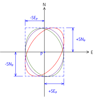 |
| Figure G-8 Many, Many Tangent Ellipses |
The standard error ellipse is the one which maximizes the semi-major axis, a, and minimizes the semi-minor axis, b, Figure G-9.
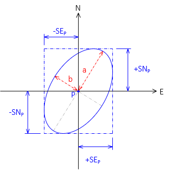 |
| Figure G-9 Standard Error Ellipse |
b. Determining Parameters
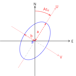
The semi-major axis is the direction in which the adjusted position is weakest, it is strongest in the semi-minor direction. These directions define the auxiliary U-V axis system, Figure G-10. AzU is the azimuth from North of the U axis.
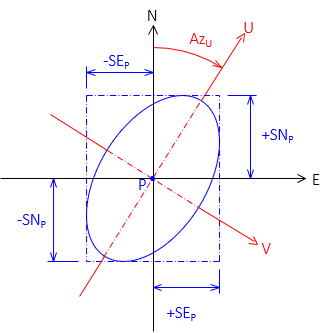 |
| Figure G-10 U-V Axis System |
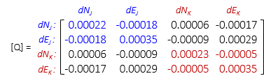
The covariance matrix, [Q], of a horizontal network can be viewed as a series of square 2 x 2 sub-matrices corresponding to each adjusted point, Figure G-11.
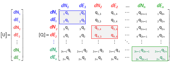 |
| Figure G-11 Unknowns and Covariance Matrices |
Note: Structure of the sub-matrices depend on the coefficients arrangement in the covariance matrix. The [Q] matrix in Figure G-11 is organized by point with North then East coefficients. If their order is reversed, or they are organized by direction instead of point (ie, all East coefficients followed by all North coefficients), the sub-matrix structures will be different. The covariance matrix organization of Figure G-11 is used in this chapter.
Figure G-12 is the sub-matrix for point i.
 |
| Figure G-12 [Q] Sub-matrix |
Diagonal elements of the sub-matrix are used to determine North and East uncertainties, Equation G-1.
 |
Equation G-1 |
Off diagonal elements relate both directions for the point to each other, hence the name covariance matrix. Because [Q] is symmetric, the off diagonal elements for each point are the same.
AzU is computed from a point's covariance values , Equation G-2.
 |
Equation G-2 |
|
T : Addend based on quadrant; Table G-1 |
|
| Table G-1 |
 |
Each adjusted point has a covariance matrix, [Φ], oriented to the U-V system. Figure G-13 shows the covariance matrix structure for point i.
 |
| Figure G-13 U-V Covariance Matrix |
[Φ] diagonal elements are computed with equations G-3 through G-5.
 |
Equation G-3 |
 |
Equation G-4 |
 |
Equation G-5 |
Since only diagonal elements are used, the symmetric off diagonal element needn't be computed.
The standard error ellipse semi-major and -minor axis lengths are computed from the diagonal elements, Equations G-6 and G-7.
 |
Equation G-6 |
 |
Equation G-7 |
c. How Confident Are We?
Standard deviations in North and East each represent an estimated 68% confidence for the respective direction. But the area of the standard error ellipse only represents about 35% confidence. That will vary somewhat based on the degrees of freedom (DF).
Increasing the confidence interval (CI) increases the size of the standard error ellipse, Figure G-14.
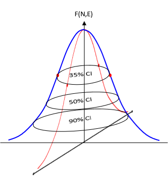 |
| Figure G-14 Confidence Intervals |
To increase confidence requires use of the F Statistic (aka, F Distribution), itself in part dependent on DF. The CI at a specific percentage is computed from Equation G-8.
| Equation G-8 | |
|
F: F Statistic modifier |
|
A common interval used by surveyors is 95%. Modifiers for 95% CI at different DF are listed in Table G-2.
| Table G-2 F Statistic |
 |
Most statistic and survey adjustments textbooks have F Statistic lookup tables for other CI and DF combinations.
3. Example
From the adjusted network of Chapter E Section 6, Figure G-13, determine the standard error ellipse and 95% CI for each adjusted point.
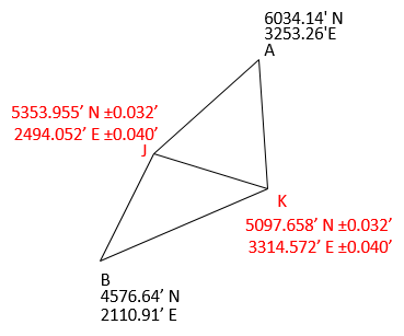 |
| Figure G-13 Adjusted Network |
The network had three DF and a So of ±2.136'. The last covariance matrix was:
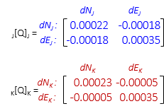
a. Sub-Matrices
b. AzU of Each Error Ellipse
Point J

Point K

c. Rotated Covariance Matrices Diagonal Elements
Point J

Point K

d. Standard Error Ellipse Parameters
Point J

Point K

e. 95% CI Error Ellipse Parameters
Table G-2: At 3 DF, F Statistic = 9.55
Point J
![]()
Point K
![]()
f. Summary
| Point | AzU | a, SU | b, SV | 95% SU | 95% SV |
| J | 215°04' | ±0.046' | ±0.021' | ±0.201' | ±0.092' |
| K | 199°54' | ±0.041' | ±0.031' | ±0.179' | ±0.135' |