{KomentoDisable}
E. Contours: Creation
A contour map is a visual surface model of the terrain. Contours are an end product in traditional paper-based metric mapping. In digital mapping, contours are one way to display the three dimensional model. Whether manual or digital, the general process to create contours is similar.
A major difference between the two environments is understanding what contours are. Manual compilation puts them in control of the mapmaker who knows what contours represent and consequently what they can and cannot do. To software, contours are complex curves consisting of mathematical graphic elements. Left to itself, software can generate contours which violate their basic characteristics. Software is only a tool for faster data manipulation and requires a knowledgeable user to ensure a correct final product. This chapter describes the contouring process in manual terms providing a new user the knowledge to create a correct contour representation in either environment.
Surface model representation resolution depends on its purpose and the accuracy of data used. A later chapter will cover data acquisition methods including collection decisions based on accuracy needs.
1. Data Points
A surface model generally begins with data points whose horizontal position and elevations are known. These can be spot elevations which are general terrain points where ground slopes change, or they could also represent features, such as street edges, property corners, ditch lines, etc. Some feature points have an effect on the surface model while others do not.
2. Interpolation
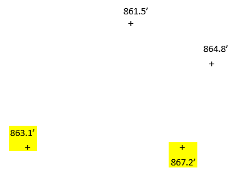
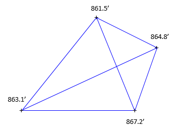
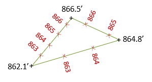
The ground slope between any two data points is assumed uniform which allows interpolation between them to locate contours. Figure E-1 is a subset of four three-dimensional (3D) data points.
 |
| Figure E-1 Data Points |
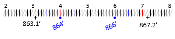
Each point is plotted at its horizontal location, indicated by the + symbol, and labeled with its elevation. The data will be used to create a two foot contour interval representation.
Starting with the two highlighted southern points, the 864 ft and 866 ft contour lines pass somewhere between them. Since a uniform slope is assumed, 864 ft and 866 ft would cross at proportional distances between the data points.
To interpolate:
The elevation difference is 867.2-863.1 = +4.1 ft
Measure the distance between the points, call it D.
From the 863.1 ft point to 864 ft:
Elev diff = 864-863.1 = +0.9 ftFrom the 863.1 ft point to 866 ft:
(dist/D) = (+0.9/+4.1); dist = (0.9/4.1)D
Elev diff = 866-863.1 = +2.9 ft
dist = (2.9/4.1)D
The interpolated points are shown in Figure E-2.
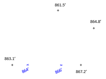 |
| Figure E-2 864 ft and 866 ft Crossings |
Additional interpolations would be done between different combinations of coordinate pairs. Figure E-3 shows the results from interpolating around the perimeter.
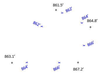 |
| Figure E-3 Perimeter Crossings |
Contour lines are drawn by connecting the respective interpolated points.
There are two issues with this method
- Lots of computations
- Interpolation pairs
Let's address these in turn.
3. Computations
This isn't a problem if the contours are created digitally since the software is performing all the computations.
However, for manual contours creation, measurements and computations are very time consuming. There are traditionally two ways to speed up the process.
a. Variable scale
A variable scale is one whose division spacing can be altered. The scale is usually a spring with its coils as the divisions. Generally every fifth and tenth coil are alternately colored. As the spring is stretched or compressed, coil spacing changes uniformly, Figure E-4.
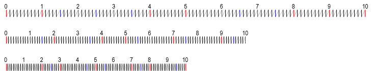 |
| Figure E-4 Variable Scale Behavior |
The spring is mounted on a rigid frame with a straightedge. It is laid between two points and the scale adjusted to match the elevation readings at each point. Intermediate points can then be accurately plotted. In Figure E-5, the scale is adjusted so the 3.1 division is on 863.1 and 7.2 division is on 867.2.
 |
| Figure E-5 Using a Variable Scale |
864 is plotted at 4 and 866 at 6. No measuring, no comps.
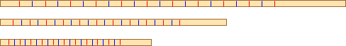
Variable scales are few and far between and expensive when found. An inexpensive, and effective, alternative, is a rubber band. The rubber band is stretched over a 10-scale and marked every 1/2 inch with an ink pen (alternating colors works well), Figure E-6.
 |
| Figure E-6 Making a Variable Scale |
Removing the rubber band will return it to its original size and the divisions will get closer together uniformly. It behaves like a variable scale when stretched, Figure E-7.
 |
| Figure E-7 Rubber Band Behavior |
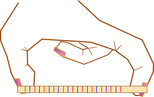
An easy way to use the rubber band is to stretch it over the thumb and index finger of one hand, Figure E-8.
 |
| Figure E-8 Using a Rubber Band Variable Scale |
Flexing the fingers will vary the scale.
b. Estimation
Because plotted distances are so short, most people can quickly estimate interpolated positions. This is fast and generally accurate enough for the map's purposes. This is the method most manual mappers employ.
4. Interpolation Pairs
Which point pairs should be used for interpolation? There are six possible interpolation paths, Figure E-10, for the four point data set of Figure E-1.
 |
| Figure E-10 Interpolation Paths |
As more data points are added, the number of interpolation paths grows geometrically. How many are enough?
Another issue is the ground slope between points. Can it be assumed uniform along every path? Consider the modestly sized data set in Figure E-12.
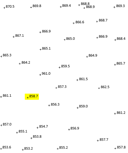 |
| Figure E-12 Area Data Set |
The 858.7 data point (highlighted) will anchor one end of multiple interpolation paths, many of which are shown in Figure E-13.
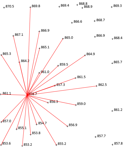 |
| Figure E-13 Interpolations from 858.7 |
While uniform slopes to nearby points are reasonable, that's not the case for points further away. Data collection in the field takes into account terrain in the data point's vicinity. Consider the northernmost 896.8 point: it was not selected based on the 858.7 data point. It's also highly unlikely the ground is uniform between points that far apart.
Using a point's nearest neighbors makes the most sense, Unfortunately, what constitutes "nearest" differs based on data density variation across the entire data set. It's also hard to program in software.
Fortunately, there is a systematic way to determine which data pairs to use: Triangulated Irregular Networks (TIN).
5. TIN
a. Triangulation
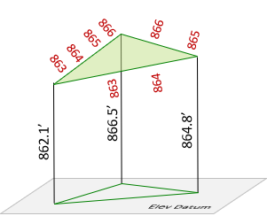
A TIN is a network of non-overlapping triangles connecting data points. Each triangle defines uniformly sloped interpolation paths along its sides, Figure E-14(a). The triangle is a 3D planar surface defined by each vertex position, Figure E-14(b).
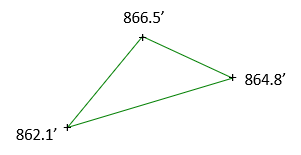 (a) Top View |
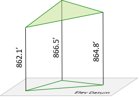 (b) Perspective View |
| Figure E-14 Data Triangle |
|
Figure E-15 Shows 1 ft interval elevations interpolated along triangle sides.
 (a) Top View |
 (b) Perspective View |
| Figure E-15 Interpolated Elevations |
|
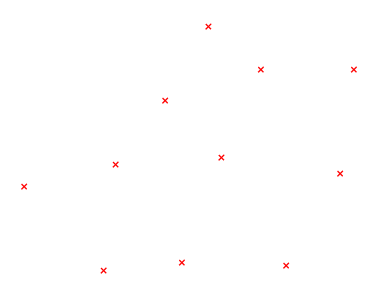
Because each is a planar surface, triangles cannot overlap. Figure E-16(a) is a data point set; Figure E-16(b) is a set of triangles connecting the data points.
 |
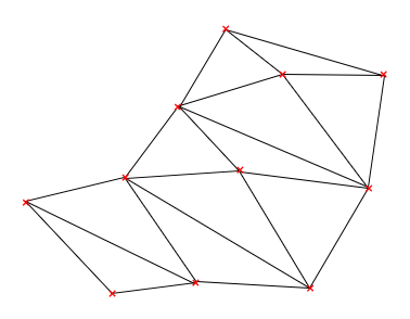 |
| (a) Data Points | (b) TIN |
| Figure E-16 TIN Creation |
|
Various combinations of non-overlapping triangles can be constructed. How do we decide which to use? An equilateral triangle is geometrically strongest, however data distribution doesn't always allow these to be uniformly created. Manual TIN creation builds the network visually - what looks strongest. Software uses algorithms to analyze different networks and select the geometrically strongest.
But both can fall flat on their face if they don't account for particular terrain features.
b. Breaklines
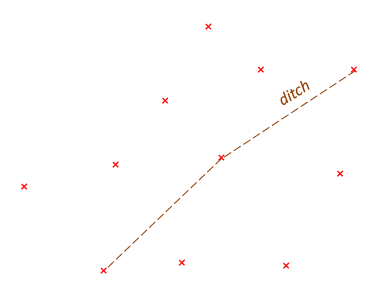
There are topographic features which affect surface model configuration. These must be included or the terrain model will be incorrect. A ditch runs through the data set in Figure 17(a). Figure 17(b) shows what happens if the ditch is ignored.
 |
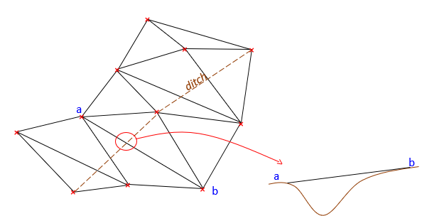 |
| (a) Ditch | (b) Interpolation Issue |
| Figure E-17 Topographic Feature |
|
Points a and b are on opposite sides of the ditch. Because the TIN connects them with a triangle side, it treats the ground as uniformly sloped between them. The ditch disappears between points a and b. The same happens wherever a triangle side crosses the ditch, which happens five times in Figure E-17(b).
Interpolation should be forced along the ditch instead of across it. The TIN is reconfigured so successive ditch line segments form one common side of two adjacent triangles, Figure E-18.
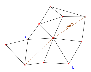 |
| Figure E-18 Interpolating Along the Ditch |
The TIN is created taking into account the ditch feature as a breakline. A breakline is a feature whose integrity must be maintained because it affects the terrain model. Feature examples that should be defined as breaklines include pavement edges, building footprints, ridges, waterways, etc. Breaklines can be man-made or natural, linear or area features.
6. Example Contour Creation
The topographic data in Figure E-19 will be used to create one foot contours.
 |
| Figure E-19 Topographic Data |
An initial TIN is created, Figure E-20.
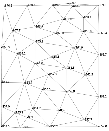 |
| Figure E-20 Initial TIN |
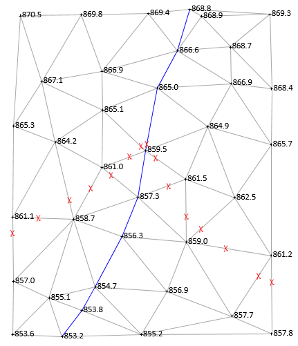
A stream runs north to south through the area. In a few places, the TIN crosses the stream, highlighted in Figure E-21.
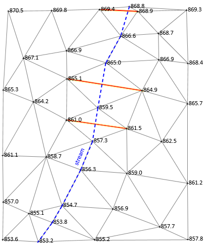 |
| Figure E-21 TIN-Stream Issues |
If the stream isn't accounted for, we could wind up with a model where water runs uphill and down.
Using the stream as a breakline, the TIN is reconfigured to go along it, Figure E-22.
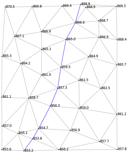 |
| Figure E-22 Final TIN with Breakline |
Once the breakline is incorporated into the TIN, interpolations can begin. In this example, we will start by putting in the 861 ft contour line.
861 ft enters the area on the west side between 861.1 and 857.0, shown with a red X in figure E-23.
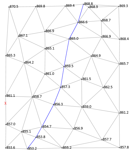 |
| Figure E-33 Starting 861 ft Contour Line |
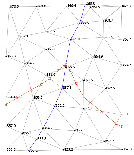
A contour line enters a triangle on one side and must exit on a second. The line cannot cross the same side of a triangle more than once and it cannot cross all three sides. 861 must exit between 861.1 and 858.7, Figure E-24.
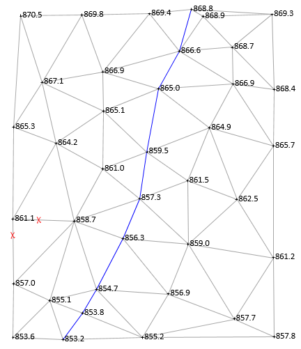 |
| Figure E-24 Second 861 ft Contour Point |
The process continues: enter a triangle on one side, exit on another; until the map edge is reached or the contour closes on itself, Figure E-25.
 |
| Figure E-25 All 861 ft Contour Points |
When all interpolated positions have been determined, they are connected with straight line segments, Figure E-26.
 |
| Figure E-26 861 ft Contour Line |
Why straight line segments? Remember that each triangle is a flat 3D surface so from one edge to another is a straight line.
Each contour is similarly created: interpolate along triangle sides, then connect with straight lines. Adjacent contours tend to have similar configurations. In Figure E-27, the 860 ft and 862 ft contours have been created on both sides of 861 ft.
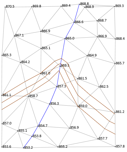 |
| Figure E-27 Adjacent Contours |
All three contours are similar. Also note their shape crossing the stream: V-shaped with the point of the V oriented upstream.
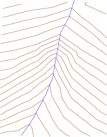
The remainder of the contours are drawn, Figure E-28.
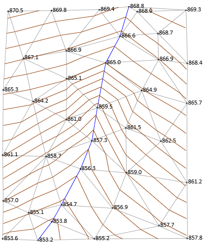 |
| Figure E-28 All Contours Drawn |
Figure E-29 are the contours with the TIN and points removed.
 |
| Figure E-29 Contours with TIN and Points Removed |
The final version, Figure E-30, is cleaned up by editing and smoothing the lines a bit, darkening and labeling index contours and the stream.
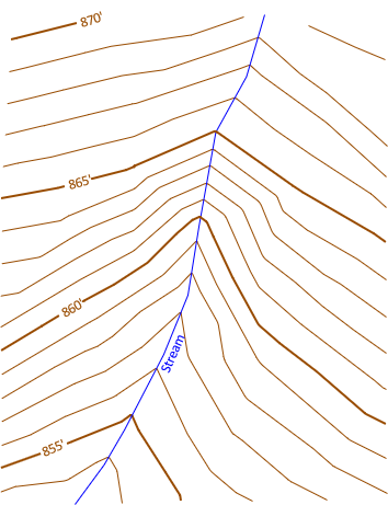 |
| Figure E-30 Final Clean contours. |
Smoothing contours is done to make them more natural looking. Except along man-made features, we don't expect them to be a series of straight line segments. However, over-smoothing, particularly in software, can cause problems: close contours lines may be bent enough to cross. The denser the data, the shorter the segments, and the more natural looking without (or with minimal) smoothing.
7. Non-Topographic Points
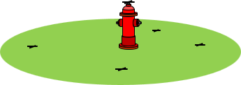
Some data points should not be included in the TIN because they do no affect terrain configuration. These points are collected primarily for planimetric purposes - horizontal location. A good example is a fire hydrant. The top of the hydrant is measured to establish its horizontal location and map an underground water line.
Figure E-31 shows five data points, four which are ground points, the fifth a fire hydrant top.
 |
 |
| (a) Top | (b) Perspective |
| Figure E-31 Five Data Points |
|
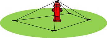
Figure E-32 shows a TIN which includes the hydrant.
 |
 |
| (a) Top | (b) Perspective |
| Figure E-32 TIN With All Points |
|
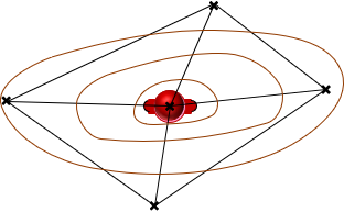
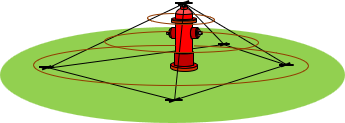
Because the hydrant is part of the TIN, contours are created towards its top, Figure E-33.
 |
 |
| (a) Top | (b) Perspective |
| Figure E-33 Phantom Contours |
|
These are phantom contours because they do not really exist.
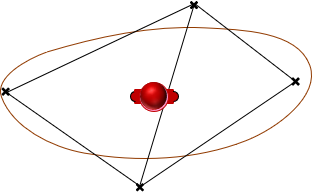
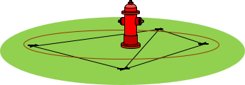
The hydrant should not be included in the TIN, Figure E-34, to prevent it affecting the terrain model.
 |
 |
| (a) Top | (b) Perspective |
| Figure E-34 Fire Hydrant Exclusion |
|
8. Summary
Whether manual or digital, the process for creating a contour line representation of terrain is:
- Generate a TIN including breaklines as appropriate
- Interpolate along triangle edges
- Connect interpolation points to create contours
- Edit/clean/label