{KomentoDisable}
D. Stadia
1. Principle
Stadia is a second tacheometric distance determination method. It has a long history in surveying and was one of the most extensive early topographic mapping methods. A few of the more interesting implementations will be discussed in this chapter to give some historical context. Despite stadia being largely replaced by newer distance measurement technologies, even contemporary instruments still have stadia corosshairs.
The stadia crosshairs, aka stadia wires, are equally spaced above and below the horizontal crosshair on an instrrument's reticule, Figure D-1.
 |
| Figure D-1 Stadia Crosshairs |
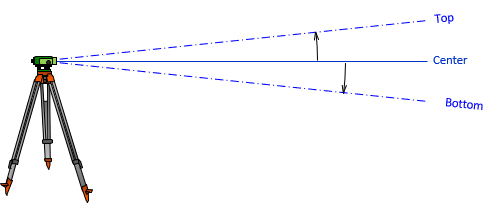
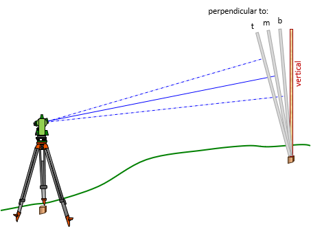
The line of sight (LoS) of the top hair is the same angle above the central LoS as the lower LoS is below it, Figure D-2.
|
|
| Figure D-2 Multiple Lines of Sight |
The difference between the top and bottom stadia hair readings on a level rod is the stadia interval, i. The interval in Figure D-3 is (7.66-6.98)=0.68.
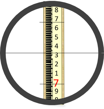 |
| Figure D-3 Stadia Interval |
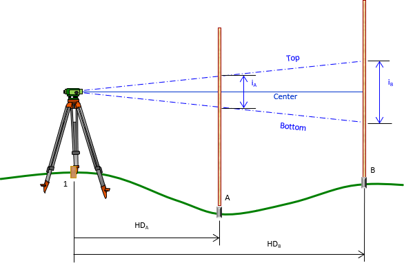
The further away the rod, the greater the interval, Figure D-4.
|
|
| Figure D-4 Interval-Distance Relationship |
The distance to the rod is the product of the rod interval and the instrument's stadia multiplier, k, Equation D-1.
 |
Equation D-1 |
The multiplier is determined by the stadia and center cross hair spacings.
Older instruments with external focusing telescopes had variable optical geometry and required an additive constant C, Equation D-2. For most instruments C was 1.
 |
Equation D-2 |
All modern instruments being internal focusing do not need a constant, and most have a multiplier of 100, making the math simple.
2. Application
Instruments using stadia can be divided into two categories:
- Fixed horizontal telescope
- Telescope that rotates in vertical plane
a. Fixed horizontal telescope
This category is made up of levels: Dumpy, Wye, and automatic.
A vertical rod will be perpendicular to the center LoS. The top and bottom LoSs should intersect the rod the same distance (half-interval) above and below the center LoS. This helps isolate reading errors. For example, the top, middle, and bottom readings in Figure D-3 are 7.66, 7.32, and 6.98. The top half-interval is (7.66-7.32)=0.34, the bottom half-interval is (7.32-6.98)=0.34. The average of the three readings is (7.66+7.32+6.98)/3 = 21.96/3 = 7.32. The half-intervals and average may differ sightly because of random reading errors, but any large differnce means there is a mistake.
Because their telescopes are limited to horizontal, stadia with levels is limited over rolling terrain. In Figure D-5, all three LoSs do not intersect the rod if the point sighted is too low or too high.
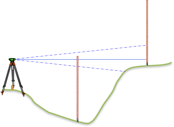 |
| Figure D-5 Level Stadia Limitations |
Technically, in both cases of Figure D-5, the half-interval can be determined using the two cross hairs that intersect the rod. These half-intervals can be doubled then multiplied by the stadia multiplier to compute the horizontal distances. The drawbacks are: (1) any error in the half-interval is doubled (2) reading mistakes can't be trapped.
Stadia with levels is generally limited to (1) balancing backsight and foresight distances and (2) measuring distances to use for proportional level circuit adjustment. These are both more fully discussed in the IV. Elevations topic.
b. Telescope that rotates in vertical plane.
(1) Geometry
Instruments in this category are alidades, transits, theodolites, and total stations. A rotating telescope provides greater flexibility allowing distance measurement along sloped surfaces, Figure D-4. Equation D-1 results in a slope distance with an inclined or depressed telescope. To reduce slope to horizontal requires measurement of the vertical or zenith angle and Equation D-1 modified to Equation D-2 or D-3.
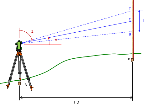 |
| Figure D-4 Rotated Telescope |
 |
Equation D-2 |
 |
Equation D-3 |
Another advantage of a rotating telescope is the ability to determine vertical distances to points substantially above or below the horizontal center LoS of a level. This allows elevation determination by trigonometric methods. Figure D-5 and Equations D-4 through D-6.
 |
| Figure D-5 Elevation Determination |
 |
Equation D-4 |
 |
Equation D-5 |
 |
Equation D-6 |
HI and HR in Equation D-6 are the instrument height and center cross hair reading on the rod, respectively. Sighting the HI on the rod simplifies Equation D-6 since HI and HR cancel.
On inclined or depressed sights, the center LoS is not perpendicular to the rod and is not in the center of the rod interval. In Figure D-4, the top half-interval is larger than the bottom half-interval, in Figure D-5 that is reversed. The greater the inclination or depression, the greater the difference between half-intervals. The difference should be relatively small, a large difference is still an indication of a possible reading mistake.
(2) Alidade
Much of the early US topographic mapping was accomplished with alidades on plane tables and later with transits, all based on stadia principles.
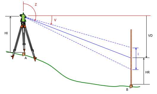
An alidade is a telescope with an abbreviated vertical circle (Beaman arc) mounted to a graduated straightedge parallel with the vertical plane of the telescope, Figure D-6.
|
|
| Figure D-6 Alidade |
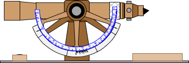
The alidade sat on a plane table which was basically a drafting table mounted to a tripod and oriented over a point. A sheet of paper was mounted on the plane table, Figure D-7.
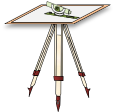 |
| Figure D-7 Alidade and Plane Table |
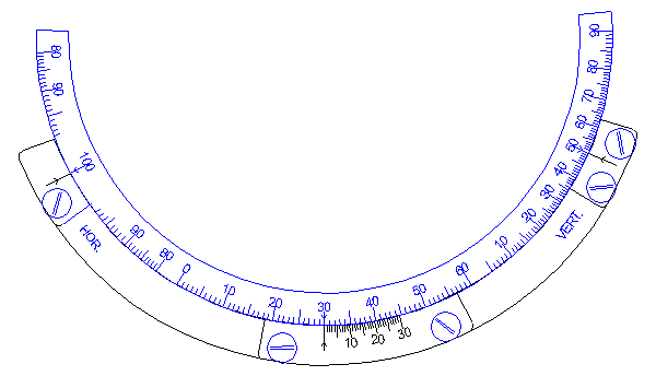
The Beaman arc is a special version of a vertical circle with logarithmic scales allowing faster stadia computations in the field without reverting to trig tables (this was waaaay before calculators and smart phones). Figure D-8 shows examples of two different Beaman arcs.
 |
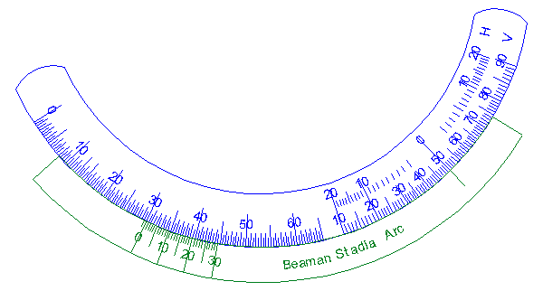 |
| Figure D-8 Beaman Arc Examples |
Stadia readings were made to a stadia board held on a point. Once the distance was computed, the point would be plotted on the paper using the alidade's scale. In this way, the initial draft of a map was compiled directly in the field.
A stadia board, Figure D-9, is simply a wider level rod with distinct division markings making readings easier at long distances.
 |
| Figure D-9 Stadia Board Portion |
(3) Self-reducing tacheometry
A major difference between transits and theodolites is the latter uses glass horizontal and vertical circles in the place of metal ones. The angle reading system is optical, using light internal to the instrument to project the circle readings to an auxillary eyepiece. Prior to the advent of total stations, a few manufactures developed a special theodolite model called a self-reducing tacheometer. These used a secondary glass circle on which were curves lines. One set of lines was plotted according to horizontal stadia distance reduction, the other according to vertical stadia distance reduction. These where projected into the field of view in place of fixed stadia crosshairs.
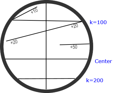
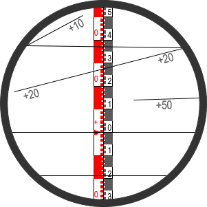
Figure D-10 is the view through the eyepiece of a self-reducing tacheometer. The center crosshair is actually below the center of the view. The top stadia hair has a 100 multiplier for the difference between it and the center hair rod readings; the bottom has a 200 multiplier. The numbered diagonal lines are multipliers for elevation differences (the numbers appear in the field of view)
 |
| Figure D-10 Self Reducing Tacheometer View |
As the telescope is inclined or depressed, the spacing between the stadia hairs changes and different vertical reduction lines move across the field of view.
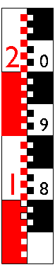
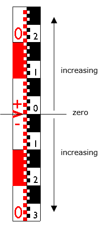
The 0 reading on the stadia board is 4 to 5 feet above the bottom. Numbering increases above and below it, Figure D-11.
 |
| Figure D-11 Stadia Board |
The board generally has an extension foot that allows adjusting the 0 mark to the instrument's height. When sighting, the center crosshair is placed on the 0 mark which makes makes interval calculation simple. Figure D-12 shows a stadia board sighting.
 |
| Figure D-12 Example Reading |
To determine the horizontal distance:
Top hair reading is 0.37; distance is 0.37x100 = 37.0
Bottom hair reading is 0.19; distance is 0.19x200 = 38.0
The bottom reading serves as a check or can be used if the top stadia hair is above the rod.
To determine elevation
+20 line crosses at reading 0.28; vertical distance is 0.28x(+20) = +5.6
Because the 0 mark is at the instrument height, the elevation is the point elevation at the instrument plus the vertical distance.
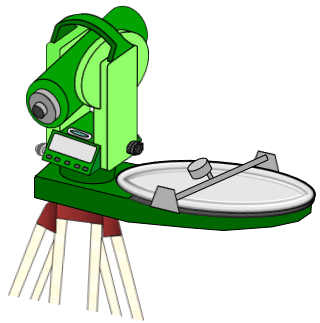
A self-reducing tacheometer could be considered the optical equivalent of an alidade. As a matter of fact, at least one manufacturer developed a special circular table on which the tacheometer was mounted. Figure D-13 is my very rough rendition of one such table.
 |
| Figure D-13 Tacheometer with Table |
The center of the circular map sheet was the instrument location. As the tacheometer was rotated horizontally, the table was geared to rotate also, keeping the map oriented correctly. A scale was attached to a rail parallel with the telescope. When the distance was determined, a marker would be slid along the rail to the scaled distance and a mark made on the map. An interesting device, but it was very quickly bypassed by development of digital measuring methods.
3. Errors
Errors have to be considered in light of expected stadia accuracy. How accurate are stadia distances? The resolution of a level rod or stadia board is is 0.01 ft and any interval will generally have 2 or 3 significant figures. The stadia multiplier (100) has 3 significant figures, trigonometric values of zenith/vertical angles have more than 3. That means a distance will have 2 or 3 significant figures.
Let's look at examples of small and large intervals, both at 70° zenith angles
| small interval | |
| i = 5.60-5.38 = 0.22 ft (2 sf) horiz dist = (0.22x100) x sin(70°) = 20.7 = 21 ft (2 sf) vert dist = (0.22x100) x cos(70°) = 7.52 = 7.5 (2 sf) |
|
| large interval | |
| i = 7.71-3.28 = 4.43 ft (3 sf) horiz dist = (4.43x100) x sin(70°)= 416.28 = 416 ft (3 sf) vert dist = (4.43x100) x cos(70°)= 151.5 = 152 (3 sf) |
|
In both cases, the horizontal distance is good to the nearest foot. Any errors less than 0.5 ft would be below stadia's "noise level".
Vertical distance accuracy is a slightly different story. For distances less than 100 feet, vertical is good 0.01 ft; over 100 ft it is good to 1 ft.
Stadia shouldn't be used for long distances considering the difficulty reading three crosshairs at those long distances. What is the practical distance limit for staida? In most cases, stadia should be limited to 300-400 ft
Taking all this into consideration, systematic errors like earth curvature and refraction are generally too small to affect stadia. That doesn't mean, however, that care shouldn't still be exercised when measuring with stadia.
a. Instrumental
(1) Multiplier
(a) Description and Behavior
The stadia multiplier for modern instruments, with a few notable exceptions, is 100. Using an incorrect multiplier is a systematic error.
(b) Compensation
Procedural: An incorrect multiplier cannot be corrected procedurally.
Mathematical: Use the multiplier determined in XV. Equipment Checks and Adjustments Chapter D. Stadia for stadia reductions.
(2) Vertical circle index
(a) Description and Behavior
The vertical circle must be correctly oriented to gravity in order to measure the correct zenith or vertical angle. A rotation in the circle causes the angle to be too large or too small by the error amount. It behaves systematically.
(b) Compensation
Procedural: Because zenith or vertical angles are not measured direct and reverse in stadia work, reversion cannot be used to compensate the error. The index error causes all angles to be too large or too small by the same amount.
Modern total stations use gravity actuated vertical circles and have axis compensation as long as the instrument is level. This compensates any potential index error.
Mathematical: If the instrument does not automatically compensate, use the vertical circle index determined in XV. Equipment Checks and Adjustments Chapter D. Stadia for stadia reductions.
b. Natural
(1) Curvature and Refraction
(a) Description and Behavior
The effect on a Line of Sight (LoS) of curvature and refraction (c&r) is discussed in Topic III. Errors E. Systematic Errors. Quick review: curvature causes high readings, refraction low; curvature is the larger error of the two.
In stadia there are three LoSs. The black lines in Figure D-14 are the "true" LoSs, red are the LoSs because of c&r. The correct stadia interval is i, the displaced interval is i(c&r).
|
|
| Figure D-14 Curvature and Refraction |
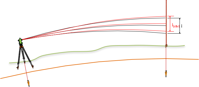
Because all three LoS are close to each other, they're each affected the same amount so the displaced stadia interval is the same as the "true" interval.
However, the vertical/zenith angle is affected which in turn affects horizontal and vertical distances. Are the differences significant? Turning it around the other way, assume a we want a zenith angle accuracy of 0°00'04". Re-arranging Equation E-1 from II. Errors E. Systematic Errors, to solve for distance:

(This only takes into account earth curvature, but it has a greater effect than refraction.)
Considering even a wide stadia board is hard to read accurately at 800+ feet, we can consider curvature (and refraction) to be inconsequential errors.
(b) Compensation
None needed.
(3) Atmospheric distortion
(a) Description and Behavior
The atmospheric correction and refraction are based on an assumption that the atmosphere is either uniform or changing uniformly along the signal path. This is not always the case. Consider the atmosphere immediately above an asphalt surface on a sunny day - the heat emitted by the surface causes a local atmospheric anomaly which affects the signal path. Almost any surface will have a boundary layer of atmospheric disturbance if it has been subject to sunlight.
(b) Compensation
The effect of atmospheric anomolies can only be minimized or eliminated by not measuring through them although this isn't always practical. Strategies can include measuring on a cloudy day or early morning.
c. Personal
(1) Instrument set up
(a) Description and Behavior
Although horizontal and vertical stadia distances are less accurate than those determined by contemporary technologies, instrument setup errors still affect measurement quality. In total, the overall effect behaves randomly.
(b) Compensation
Careful setup and experience.
(2) Instrument height determination
(a) Description and Behavior
Using an incorrect instrument height will not affect horizontal or vertical distances. It will, however, affect elevations determined using Equation D-6. Incorrect instrument height is an additive systematic error.
(b) Compensation
Care should be exercised measuring instrument height, generally using a cloth tape or pocket rod.
(3) Level rod
(a) Description and Behavior
The level rod or stadia board must be held vertical or a systematic error will be introduced reading the rod interval
(b) Compensation
The only way to compensate is to hold the rod vertical using a rod bubble. Waving the rod, as in differential leveling does not work. The minimum reading for each crosshair occurs when the rod is perpendicular to each respective LoS, Figure D-15.
 |
| Figure D-15 Waving Rod Error |
(4) Parallax
(a) Description, Behavior, and Compensation
Parallax and its compensation are described in I. Basic Principles Chapter E. Bubbles, Axes, and Optics, Oh My! Its behavior is random.
(5) Reading errors
(a) Description and Behavior
Three crosshairs and a vertical angle are read by the instrument operator. Reading errors are random.
(b) Compensation
Careful field procedures; checking half-interval equality.
(6) Recording errors
(a) Description and Behavior
Mistakes.
(b) Compensation
Careful recording, verifying readings.
(7) Computations
(a) Description and Behavior
Mistakes
(b) Compensation
Careful computations.