{KomentoDisable}
C. Meridian Conversion
1. What
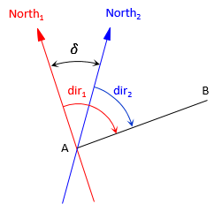
A meridian conversion is converting the direction of a line from one meridian reference to another, Figure C-1.
 |
| Figure C-1 Converting Directions |
The conversion consists of adjusting the direction of a line by the angle between the two meridians.
2. Magnetic Direction Conversion
a. Magnetic Meridian
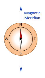
Directions and angles for early land surveys were measured using a compass which is referenced to magnetic north. Unlike many other meridians, magnetic north is relatively easy to establish in the field: just hold a compass level and wait patiently. When it stops swinging, the needle will be aligned with the magnetic north-south meridian, Figure C-2.
 |
| Figure C-2 Compass and Meridian |
While easy to establish, there are two major problems using magnetic directions:
(1) Poles move
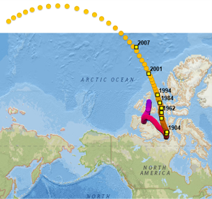
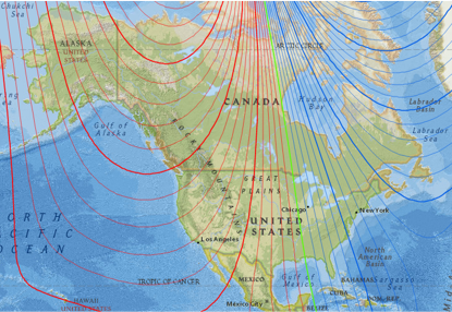
The magnetic poles move over time which affects the median direction. Figure C-3 is from NOAA National Centers for Environmental Information (https://maps.ngdc.noaa.gov/viewers/historical_declination/). It shows the magnetic north pole movement from 1590 to 2025 based on measurements and models.
The movement is neither systematic nor constant which means magnetic directions of lines change inconsistently over time.
 |
| Figure C-3 Magnetic North, 1590-2025 (from NOAA NCEI) |
(2) A magnetic meridian is not straight
Natural anomalies along the meridian affect the magnetic field causing it to change direction. Local anomalies, such as high voltage power lines and large buildings with steel superstructures, will attract the compass needle. Natural anomalies change over time and humans are constantly building stuff so the resultant meridian is neither stable over time nor mathematical.
Local anomalies can be especially problematic. The magnetic meridians at both ends of a long line may not be parallel if there is a significant local anomaly at one end. Forward and back directions may differ from simple bearing quadrant reversal and 180° azimuth difference.
Because of these issues, magnetic directions are not typically used today. But because they have been used in the past, a surveyor should understand how to convert magnetic directions to a static reference meridian.
b. Declination
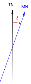
Magnetic directions are generally converted to true directions. Declination, Figure C-4, is the angle from the true meridian to the magnetic median.
 |
| Figure C-4 Declination |
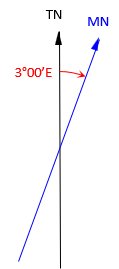
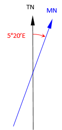
It is expressed as an angle and direction. The declination in Figure C-5(a) is 3°00' E, in Figure C-5(b) is 4°30'W.
 |
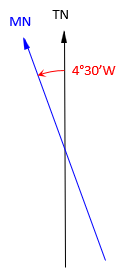 |
| (a) East | (b) West |
| Figure C-5 Declination: Angle and Direction |
|
Because magnetic north moves over time, declination changes. Variation is the rate of declination change. It is not constant over time, Figure C-6.
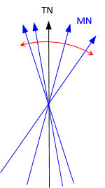 |
| Figure C-6 Declination and Variation |
Future variation can only be predicted from models based on past behavior. Variation is an annual rate stated as an angle and direction. For example, a 1°00' E variation means that in one year declination moves east 1°00'.
Isogonic lines are used to graphically depict declination behavior over an area. An isogonic line is a line of constant declination; it's the declination equivalent of a contour line. The agonic line is the line of zero declination - magnetic and true north directions coincide.
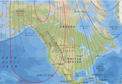
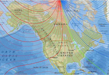
Figure C-7 are isogonic lines across North America for 2021.
 |
| Figure C-7 2021 Isogonic Lines |
The isogonic interval (difference between adjacent lines) is 2°00'; red lines are east declinations, blue are west. The green line is the agonic line.
Figure C-8 are isogonic lines across North America for 2000 across the same area.
 |
| Figure C-8 2000 Isogonic Lines |
The general pattern is similar to the map in Figure C-7 but there are differences. Note the agonic line change across the US.
The US Public Land Survey started in the 1780's. Figure C-9 shows the declinations in 1785.
 |
| Figure C-9 1785 Isogonic Lines |
Compare it to the 2000 and 2021 maps. Click here for a short video of declination change from the mid-1700s to 2021.
The maps in Figures C-7, -8, -9, and those in the video are from NOAA National Centers for Environmental Information (https://maps.ngdc.noaa.gov/viewers/historical_declination/).
c. Magnetic to True Examples
When converting between magneric and true directions, remember:
- The only thing that moves is the magnetic meridian. Even though a line's direction changes, it physically remains in its same position.
- Declination is specified for the north ends of the meridians, the magnetic south end of the meridian is off the same angle but in the opposite direction.
As simple as a meridian conversion is, the conversion is easy to apply incorrectly. A sketch helps tremendously.
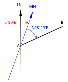
Example 1
In 1885 the declination was 5°20'E
Sketch
(a) The magnetic bearing of line AB in 1885 was recorded as N58º45’E. What is the true bearing of the line?
Sketches
 |
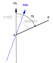 |
The true bearing angle is the sum of the magnetic bearing and deflection angles.

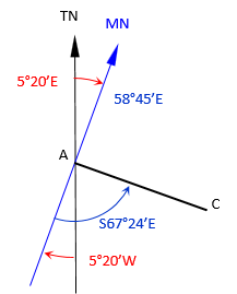
(b) The magnetic bearing of line AC in 1885 was recorded as S67º24’E. What is its true bearing?
Sketches
 |
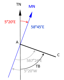 |
The true bearing angle is the difference between the bearing and deflection angles.

The declination angle is added to or subtracted from the bearing angle depending on the bearing quadrant.
Example 2
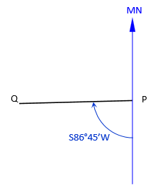
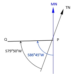
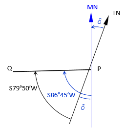
The magnetic bearing of line PQ in 1925 was recorded as S86º35’W. The present true bearing of the line is S79º50’W.
What was the declination in 1925?
Create a sketch in a series of steps
| Magnetic bearing of line PQ in 1925 was S86º35’W... | |
 |
|
| Present true bearing is S79°50'W... | |
 |
|
Come back from the line 79°50' to the east to establish the south end of the true meridian.
| What was the 1925 declination? | |
 |
|
The declination is the difference between the two directions.
![]()
Since the north end of the magnetic meridian is west of the true meridian, the deflection is 6°55' W.
d. Surveyor's Compass
This section is not necessary for understanding delcination, but because a compass was an early angle measurement device, a brief description of it is included for some historical context.
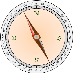
When you look at the face of a traditional surveyor's compass, Figure C-10, you'll see that East and West are flipped. Huh, what's up with that?
 |
| Figure C-10 Surveyor's Compass |
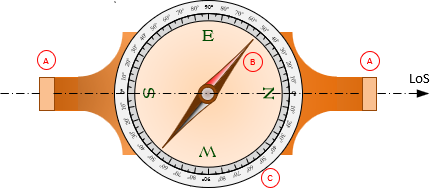
Notable compass parts are, Figures C-11 and C-12:
- A - Sighting vanes (later replaced with a telescope)
- B - Magnetic needle
- C - Angle divisions
 |
| Figure C-11 Surveyor's Compass - Top View |
 |
| Figure C-12 Surveyor's Compass - Side View |
Early compasses used a simple sighting system consisting of two upright vanes at the front and rear. A slit in each vane, aligned with the N and S compass marks, allowed the surveyor to sight on a point or target, Figure C-13.
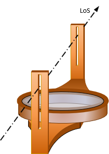 |
| Figure C-13 Surveyor's Compass - Perspective View |
Later instruments included first a fixed telescope, then one which rotated in a vertical plane. The compass lead to the transit which led to the theodolite which led to the total station... Most contemporary total stations include a tubular compass maintaining an evolutionary tie to the surveyor's compass.
The compass card is divided into four numbered quadrants. Each is numbered beginning with 0° at N and S, increasing to 90° at E and W, Figure C-14.
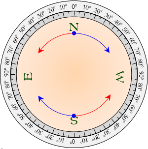 |
| Figure C-14 Compass Card |
The reversed east and west markings with the 0°-90° angle quadrants allow direct reading of a line's magnetic bearing.
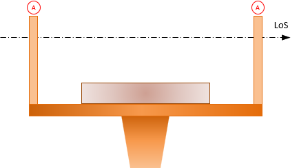
The entire instrument is rotated to sight a point or target. The needle is free to swing, always pointing along the magnetic meridian, as the compass is rotated. When the aligned with the needle, Figure C-15, the LoS is either directly north or south.
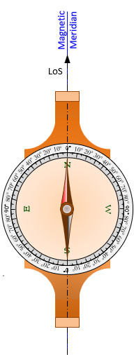 |
| Figure C-15 Sighting Along Meridian |
To determine the bearing to another point, the compass is rotated to sight it, Figure C-16.
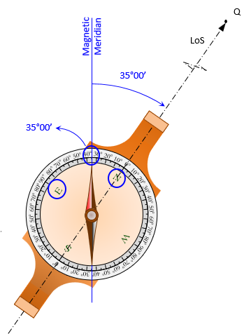 |
| Figure C-16 Magnetic Bearing to Point Q |
The north end of the needle is used to read the bearing angle and quadrant. The needle points at the bearing angle and its north end falls between the letters identifying the quadrant The magnetic bearing to point Q in Figure C-16 is N 35°00' E.
Sighting point R, Figure C-17,...
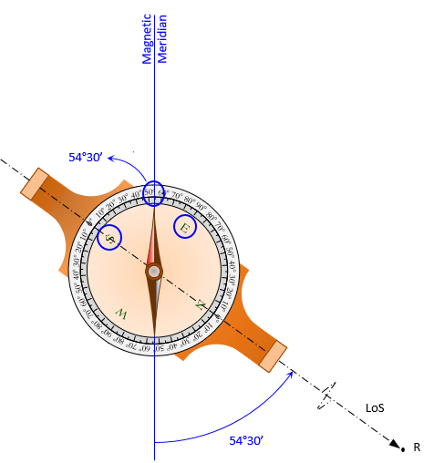 |
| Figure C-17 Magnetic Bearing to Point R |
... the magnetic bearing to it is is S 54°30' E. The north end of the needle is used to read the bearing.
By flipping East and West on the compass, bearings can be read directly without having to do any math. Neat, huh?
3. Adjacent Survey
Not all surveys are referenced to a formal meridian. Some surveyors assume the direction of one line which serves as the basis for the remaining lines. As long as the survey stands alone and otherwise meets it objectives (eg, parcel area, physical line locations, etc), an assumed direction is fine. However, if the survey will be integrated with others, they must all have the same direction reference.
This can happen when two adjoining parcels are surveyed by different surveyors at different times. Individually, the surveys may be high quality and meet the clients' needs. But they won't map together correctly if each used a different direction assumption - it will appear that the surveys are rotated with respect to each other..
For example:
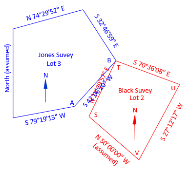
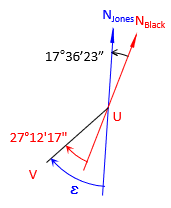
Surveyor Jones is hired to survey Lot 3 in a subdivision. Because one line runs close to north-south, he assumed its direction as North and completed his survey, His final directions after traverse adjustment are shown in Figure C-18.
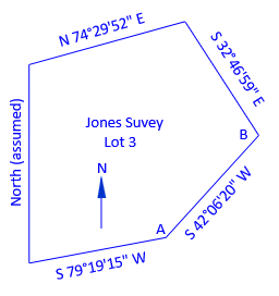 |
| Figure C-18 Jones Lot 3 Survey |
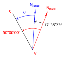
Surveyor Black surveyed Lot 2, on the southeast side of Lot 3. She started with an assumed direction of N 50°00'00" W on one line. Her final line directions are shown in Figure C-19.
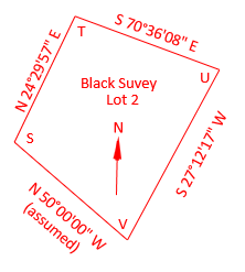 |
| Figure C-19 Lot 2 Survey |
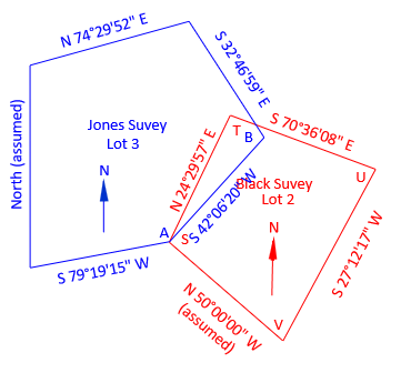
The common line between Lots 3 and 2 is Jones' line AB and Black's line ST. Because the lines have different directions in each survey, there will be a problem plotting the surveys together on a single map. Whether points B and T coincide, Figure C-20, or points A and S coincide, Figure C-21, the common line will will be rotated between surveys.
 |
| Figure C-20 Common Points B and TM |
 |
| Figure C-21 Common Points A and S |
Assuming a direction, each surveyor fixed their respective north meridians. The angle between the common lines in Figures C-20 and C-21 is the angular difference between their north meridians.
Even though Figures C-20 and C-21 show two different lines, that is not the real situation. There is only one line but two different norths, Figure C-22
 |
| Figure C-22 Meridian Difference |
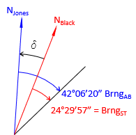
Using a single common line, we can reconstruct where the surveyors' assumed north meridians were:
- Jones' was 42°06'20" northwest of the common line
- Black's was 24°29'57" northwest of the common line.
The angle between their meridians, δ, is:
![]()
This angle is used to convert Black's directions to Jones' north meridian.
Stepping through the remaining three lines of Lot 2:
| Line TU | |
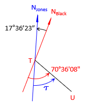 |
|
| BrngTU = S 52°59'45" E | |
| Line UV | |
 |
|
| BrngUV = S 44°48'40" W | |
| Line VS | |
 |
|
| BrngVS = N 32°23'37" W | |
4. Meridian Convergence
a. Meridian Orientation
Non-magnetic meridians are either parallel or convergent. For Plane Surveying applications over smaller areas and in assumed systems, parallel meridians are used, Figures C-24.
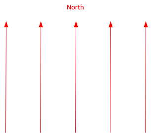 |
| Figure C-24 Parallel Meridians |
In a parallel meridian system, there is no singular unique north point.
For Geodetic Surveying applications, where the earth's shape is taken into account, Figure C-25, meridians converge to a particular north point, Figure C-26.
 |
| Figure C-25 Earth Shape |
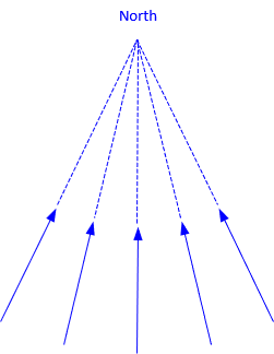 |
| Figure C-26 Convergent Meridians |
Depending on the geodetic reference system, the north point may be
- True (aka Geographic) - based on the earth's average rotational axis (the earth wobbles as it rotates).
- Astronomic - based on gravity and celestial observations (using either Polaris or the Sun).
- Geodetic - based on a particular mathematical earth model.
For purposes of this Chapter, we'll limit discussion to the northern hemisphere. In the southern hemisphere, meridians converge to a south point, reversing things by 180°.
b. Forward and Back Directions
In Chapter A. Definitions, it was stated that
- A forward and back bearing had the same angle from the meridian but opposite quadrants
- A forward and back azimuth differed by 180°
These are true only for parallel meridians. When meridians converge, the forward and back direction angles must account the convergence.
Bearings
Figure C-27 shows the geometry for the bearing and back bearing of line AB.
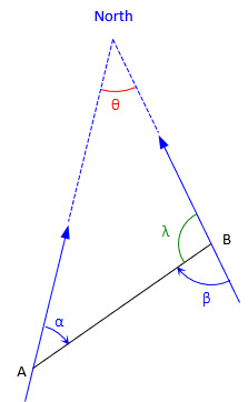 |
| Figure C-27 Forward-Back Bearing |
The forward bearing is N α E, the back bearing is S β W. The angular convergence between meridians is θ.
From the geometry in Figure C-27:
The last two equations show that the forward and back bearing angles differ by the convergence.
Azimuths
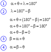
The geometry for the azimuth and back azimuth line EF is shown in Figure C-28.
 |
| Figure C-28 Forward-Back Azimuth |
The forward azimuth of line EF is ε, the back azimuth is φ. θ is the angular convergence between the meridians.
From the geometry in Figure C-19:
The last two equations show that the 180° difference between the forward and back azimuths must be adjusted by the convergence.
c. Grid Systems
A formal grid coordinate system covers an area large enough that convergence of true meridians, Figure C-29, must be taken into account.
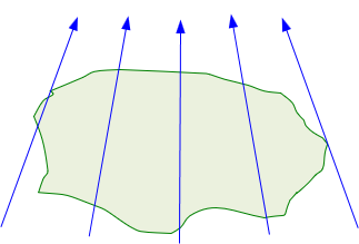 |
| Figure C-29 Converging True Meridians |
The coordinate system uses a Grid North axis and a perpendicular Grid East axis. Grid north meridians, Figure C-21, are parallel with the Grid North axis.
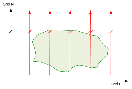 |
| Figure C-30 Parallel Grid Meridians |
Figure C-31 shows the grid meridians overlaid on the true meridians.
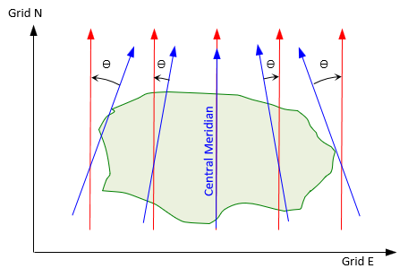 |
| Figure C-31 Varying Convergence |
The grid system is centered on the area so grid north and true north coincide along the central meridian. Moving east or west of the Central Meridian, grid meridians remain parallel while true meridians do not. The further from the Central Meridian, the greater the convergence angle.
In a grid system, convergence is from the true meridian to the grid meridian. East of the Central Meridian convergence is positve, west it is negative.
Example
The true azimuth for line RJ is 238°05'46". The convergence at point R is +1°54'21", at J it is -2°35'16".
Compute: (a) Grid azimuth from R to J, and (b) True azimuth from J to R
Sketch of provided information
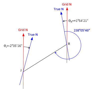
(a) Grid azimuth from R to J
Sketch
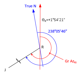
![]()
(b) True azimuth from J to R
Sketch
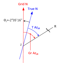
Because grid north meridians are parallel, the grid azimuths of RJ and JR differ by exactly 180°.
![]()
![]()
The difference between the true azimuths of RJ and JR is:
![]()
This is 4°29'37" greater than 180°00'00" and is the sum of the absolute values of the convergences. The effect of convergences on forward and back true directions are:
- If convergences are in opposite directions, the forward and back true azimuths differ from 180° by the sum of the convergence absolute values.
- If the convergences are in the same direction, the forward and back true azimuths differ from 180° by the difference of the convergences.